Communicated by Les Valiant .

What Size Net Gives Valid Generalization?

Eric B. Baum*
Jet Propulsion Laboratorj; California Institute o f Technology,
Pasadena, C A 91 109, EE.UU

David Haussler
Department o f Computer and Information Sciencrs,
University o f California, Santa Cruz, California 95064, EE.UU

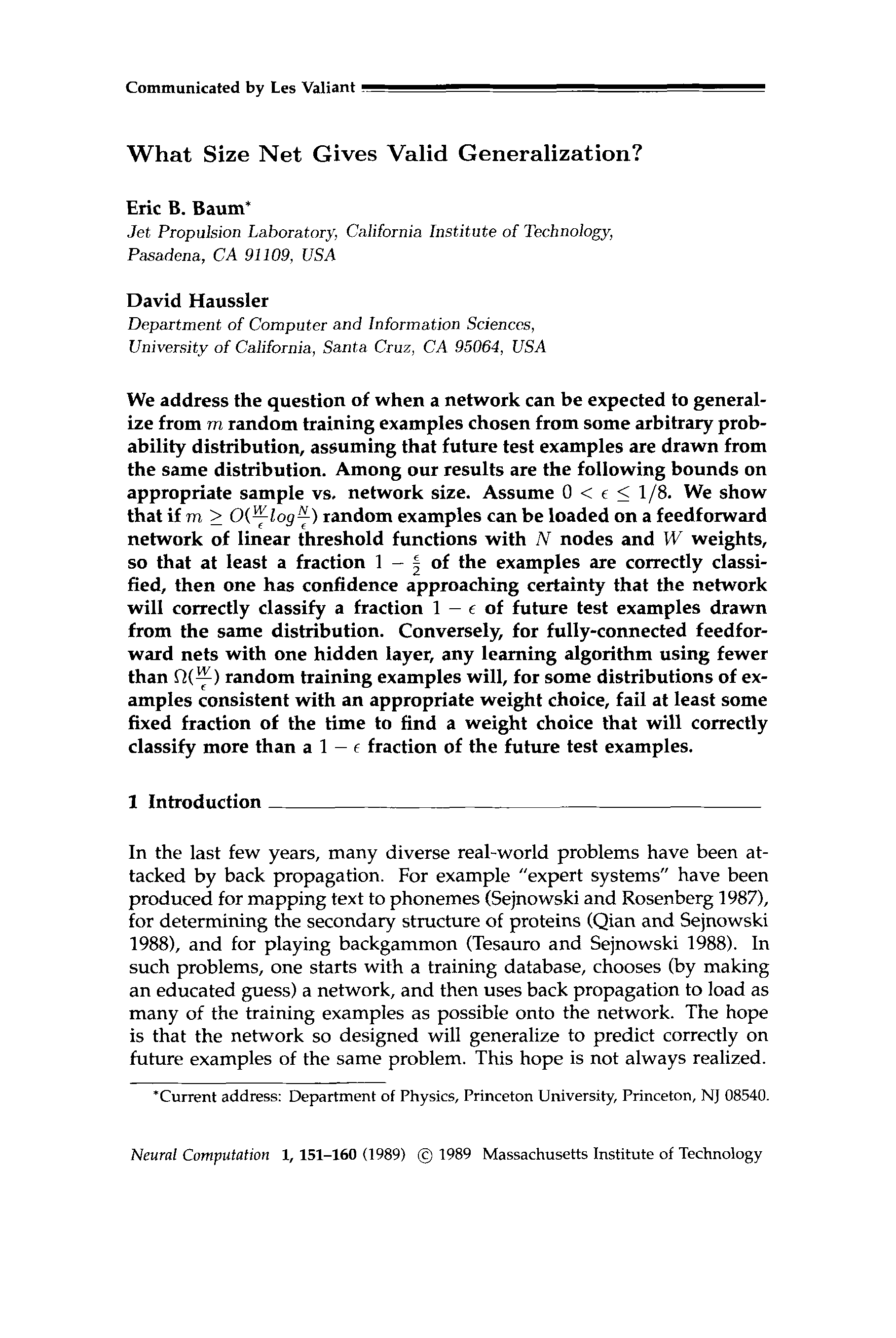
We address the question of when a network can be expected to general-
ize from m random training examples chosen from some arbitrary prob-
ability distribution, assuming that future test examples are drawn from
the same distribution. Among our results are the following bounds on
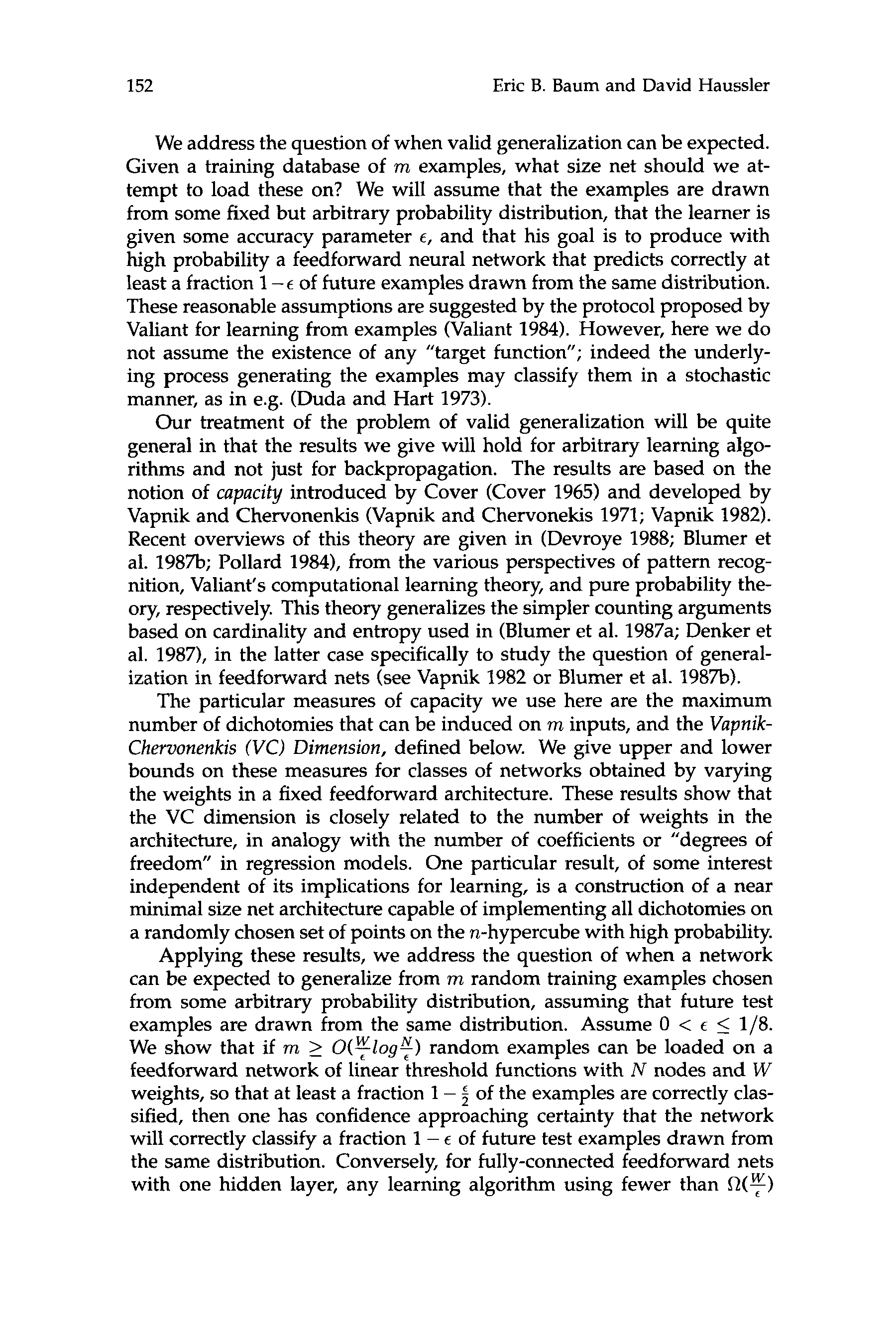
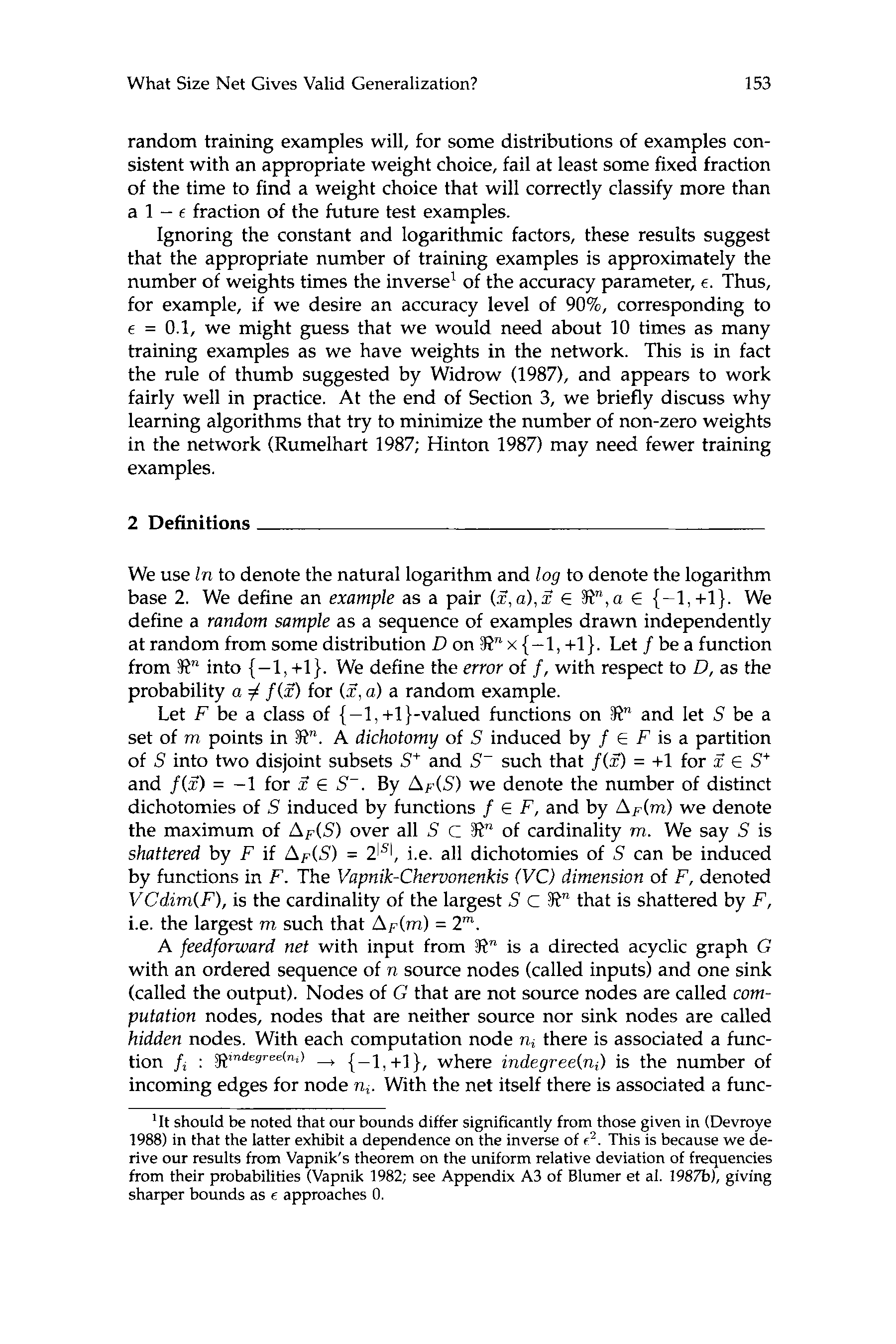
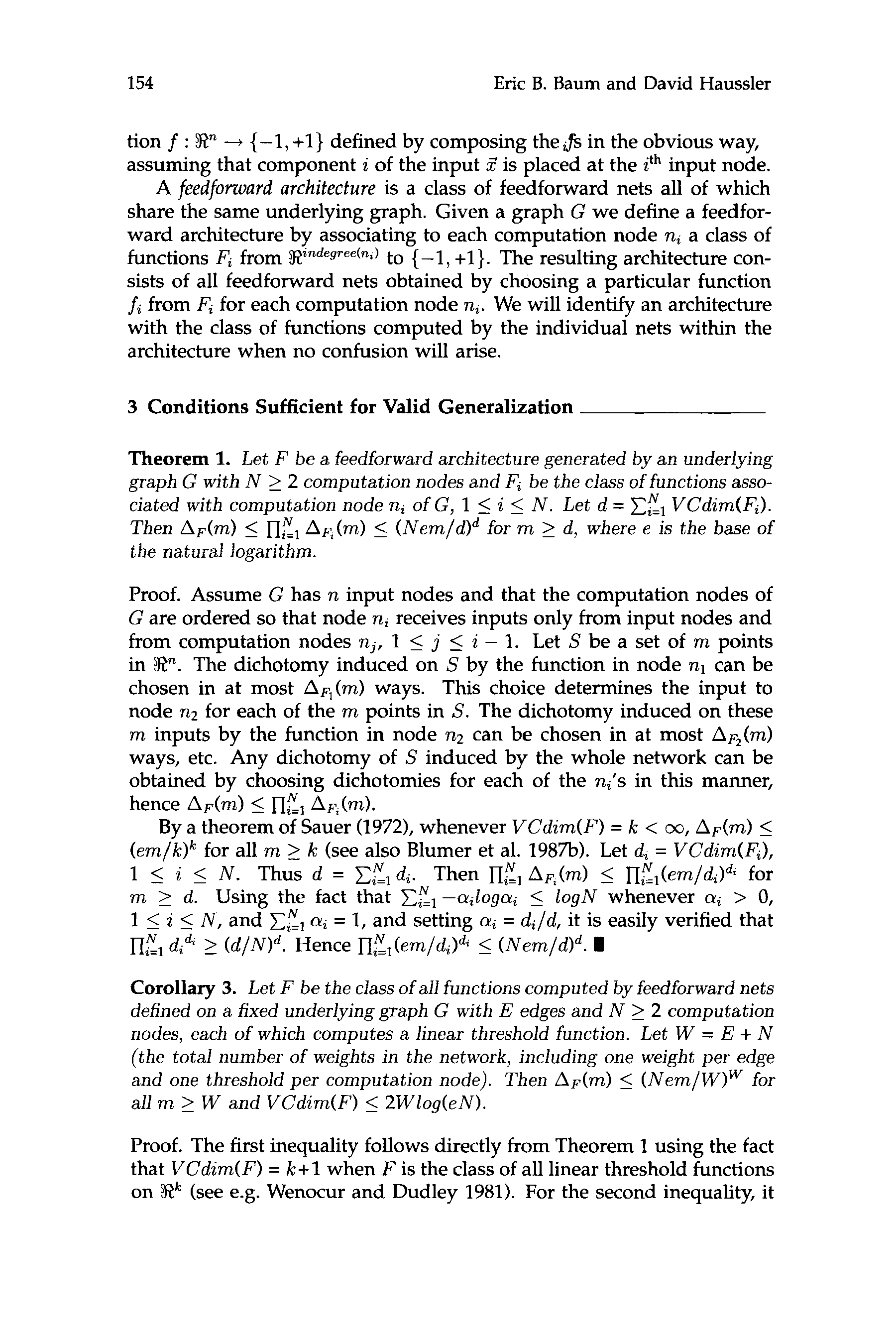
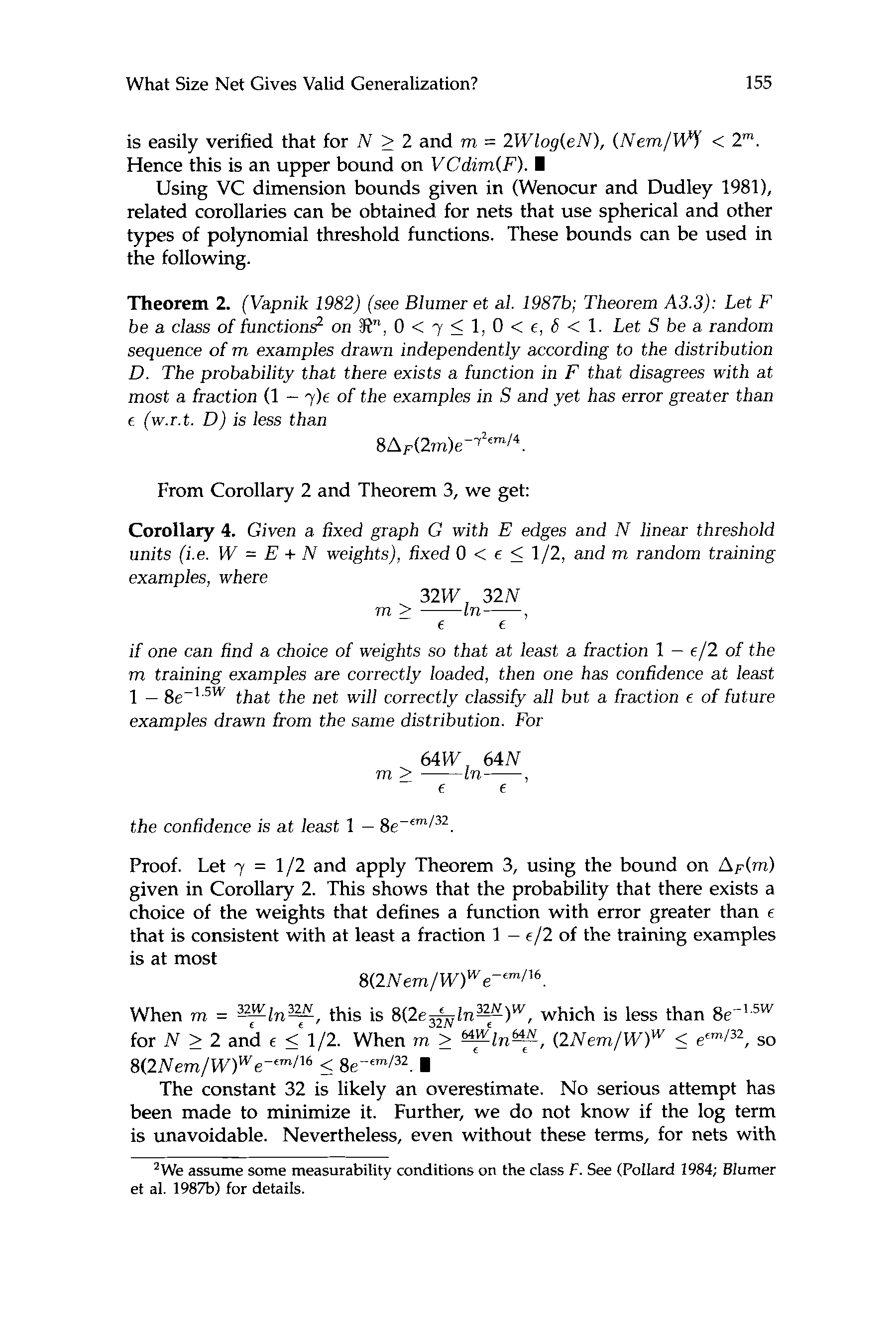
appropriate sample vs, network size. Assume 0 < E 5 1/8. We show that if m 2 0($209!) random examples can be loaded on a feedforward network of linear threshold functions with N nodes and W weights, so that at least a fraction 1 - 5 of the examples are correctly classi- fied, then one has confidence approaching certainty that the network will correctly classify a fraction 1 - E of future test examples drawn from the same distribution. Conversely, for fully-connected feedfor- ward nets with one hidden layer, any learning algorithm using fewer than O(F) random training examples will, for some distributions of ex- amples consistent with an appropriate weight choice, fail at least some fixed fraction of the time to find a weight choice that will correctly classify more than a 1 - E fraction of the future test examples. 1 Introduction In the last few years, many diverse real-world problems have been at- tacked by back propagation. For example ”expert systems” have been produced for mapping text to phonemes (Sejnowski and Rosenberg 19871, for determining the secondary structure of proteins (Qian and Sejnowski 19881, and for playing backgammon (Tesauro and Sejnowski 1988). In such problems, one starts with a training database, chooses (by making an educated guess) a network, and then uses back propagation to load as many of the training examples as possible onto the network. The hope is that the network so designed will generalize to predict correctly on future examples of the same problem. This hope is not always realized. *Current address: Department of Physics, Princeton University, Princeton, NJ 08540. Neural Computation 1, 151-160 (1989) @ 1989 Massachusetts Institute of Technology l D o w n o a d e d f r o m h t t p : / / d i r e c t . m i t . / e d u n e c o a r t i c e - p d / l f / / / / / 1 1 1 5 1 8 1 1 8 1 7 n e c o 1 9 8 9 1 1 1 5 1 p d . . . . . f b y g u e s t t o n 0 7 S e p e m b e r 2 0 2 3 152 Eric B. Baum and David Haussler We address the question of when valid generalization can be expected. Given a training database of m examples, what size net should we at- tempt to load these on? We will assume that the examples are drawn from some fixed but arbitrary probability distribution, that the learner is given some accuracy parameter E , and that his goal is to produce with high probability a feedforward neural network that predicts correctly at least a fraction 1 - 6 of future examples drawn from the same distribution. These reasonable assumptions are suggested by the protocol proposed by Valiant for learning from examples (Valiant 1984). However, here we do not assume the existence of any "target function"; indeed the underly- ing process generating the examples may classify them in a stochastic manner, as in e.g. (Duda and Hart 1973). Our treatment of the problem of valid generalization will be quite general in that the results we give will hold for arbitrary learning algo- rithms and not just for backpropagation. The results are based on the notion of capacity introduced by Cover (Cover 1965) and developed by Vapnik and Chervonenkis (Vapnik and Chervonekis 1971; Vapnik 1982). Recent overviews of this theory are given in (Devroye 1988; Blumer et al. 198%; Pollard 1984), from the various perspectives of pattern recog- nition, Valiant's computational learning theory, and pure probability the- ory, respectively. This theory generalizes the simpler counting arguments based on cardinality and entropy used in (Blumer et al. 1987a; Denker et al. 1987), in the latter case specifically to study the question of general- ization in feedforward nets (see Vapnik 1982 or Blumer et al. 1987b). The particular measures of capacity we use here are the maximum number of dichotomies that can be induced on m inputs, and the Vupnik- Chervonenkis (VC) Dimension, defined below. We give upper and lower bounds on these measures for classes of networks obtained by varying the weights in a fixed feedforward architecture. These results show that the VC dimension is closely related to the number of weights in the architecture, in analogy with the number of coefficients or "degrees of freedom" in regression models. One particular result, of some interest independent of its implications for learning, is a construction of a near minimal size net architecture capable of implementing all dichotomies on a randomly chosen set of points on the n-hypercube with high probability. Applying these results, we address the question of when a network can be expected to generalize from m random training examples chosen from some arbitrary probability distribution, assuming that future test examples are drawn from the same distribution. Assume 0 < t 5 1/8. We show that if m 1 O(:logT) random examples can be loaded on a feedforward network of linear threshold functions with N nodes and W weights, so that at least a fraction 1 - f of the examples are correctly clas- sified, then one has confidence approaching certainty that the network will correctly classify a fraction 1 - E of future test examples drawn from the same distribution. Conversely, for fully-connected feedforward nets with one hidden layer, any learning algorithm using fewer than O ( 5 ) l D o w n o a d e d f r o m h t t p : / / d i r e c t . m i t . / e d u n e c o a r t i c e - p d / l f / / / / / 1 1 1 5 1 8 1 1 8 1 7 n e c o 1 9 8 9 1 1 1 5 1 p d . . . . . f b y g u e s t t o n 0 7 S e p e m b e r 2 0 2 3 What Size Net Gives Valid Generalization? 153 random training examples will, for some distributions of examples con- sistent with an appropriate weight choice, fail at least some fixed fraction of the time to find a weight choice that will correctly classify more than a 1 - E fraction of the future test examples. Ignoring the constant and logarithmic factors, these results suggest that the appropriate number of training examples is approximately the number of weights times the inverse' of the accuracy parameter, E . Thus, for example, if we desire an accuracy level of 90%, corresponding to E = 0.1, we might guess that we would need about 10 times as many training examples as we have weights in the network. This is in fact the rule of thumb suggested by Widrow (1987), and appears to work fairly well in practice. At the end of Section 3, we briefly discuss why learning algorithms that try to minimize the number of non-zero weights in the network (Rumelhart 1987; Hinton 1987) may need fewer training examples. 2 Definitions We use In to denote the natural logarithm and log to denote the logarithm base 2. We define an example as a pair ( 2 , u ) , 2 E P , a E {-l,+l}. We define a random sample as a sequence of examples drawn independently at random from some distribution D on Sn x { -1, +1}. Let f be a function from RR into {-1, +l}. We define the errur of f , with respect to D, as the probability a + f (2) for (2, a ) a random example. Let F be a class of { -1, +I}-valued functions on Rn and let S be a set of m points in Rn. A dichotomy of S induced by f E F is a partition of S into two disjoint subsets S' and S- such that f(2) = +1 for 2 E S' and f ( 2 ) = -1 for 2 E S-. By A,(S) we denote the number of distinct dichotomies of S induced by functions f E F , and by A,(m) we denote the maximum of AF(S) over all S c Sn of cardinality m. We say S is Shattered by F if A&5') = 21'1, i.e. all dichotomies of S can be induced by functions in F. The Vapnik-Chervonenkis W C ) dimension of F , denoted VCdinz(F), is the cardinality of the largest S c Xn that is shattered by F , i.e. the largest m such that A&n) = 2". A feedforward net with input from !JIn is a directed acyclic graph G with an ordered sequence of n source nodes (called inputs) and one sink (called the output). Nodes of G that are not source nodes are called com- putation nodes, nodes that are neither source nor sink nodes are called hidden nodes. With each computation node n, there is associated a func- tion ji p n d e g r e e h , ) + {-1, +I}, where indegree(n,) is the number of incoming edges for node n,. With the net itself there is associated a func- 'It should be noted that our bounds differ significantly from those given in (Devroye 1988) in that the latter exhibit a dependence on the inverse of 6'. This is because we de- rive our results from Vapnik's theorem on the uniform relative deviation of frequencies from their probabilities (Vapnik 1982; see Appendix A3 of Blumer et al. 1987b), giving sharper bounds as c approaches 0. l D o w n o a d e d f r o m h t t p : / / d i r e c t . m i t . / e d u n e c o a r t i c e - p d / l f / / / / / 1 1 1 5 1 8 1 1 8 1 7 n e c o 1 9 8 9 1 1 1 5 1 p d . . . . . f b y g u e s t t o n 0 7 S e p e m b e r 2 0 2 3 154 Eric B. Baum and David Haussler { -1, +1} defined by composing the Zfs in the obvious way, tion f : W -+ assuming that component i of the input 2 is placed at the ith input node. A feedforward architecture is a class of feedforward nets all of which share the same underlying graph. Given a graph G we define a feedfor- ward architecture by associating to each computation node n, a class of functions F, from Pndegree(nt) to {-1, +1}. The resulting architecture con- sists of all feedforward nets obtained by choosing a particular function f, from F, for each computation node n,. We will identify an architecture with the class of functions computed by the individual nets within the architecture when no confusion will arise. 3 Conditions Sufficient for Valid Generalization Theorem 1. Let F be a feedforward architecture generated by an underlying graph G with N 2 2 computation nodes and Fi be the class of functions asso- ciated with computation node n, of G, 1 5 i 5 N . Let d = XE, VCdim(Fi). Then A,(m) 5 @, A,(m) 5 (Nem/d)d for m 2 d , where e is the base of the natural logarithm. Proof. Assume G has n input nodes and that the computation nodes of G are ordered so that node ni receives inputs only from input nodes and from computation nodes nj, 1 5 j 5 i - 1. Let S be a set of m points in $I2". The dichotomy induced on S by the function in node nl can be chosen in at most A , ( m ) ways. This choice determines the input to node n 2 for each of the m points in S. The dichotomy induced on these m inputs by the function in node n2 can be chosen in at most A,(m) ways, etc. Any dichotomy of S induced by the whole network can be obtained by choosing dichotomies for each of the ni's in this manner, hence A d m ) 5 n:, A,(rn). By a theorem of Sauer (1972), whenever VCdim(F) = k < 03, A,(m) 5 (em/k)k for all m 2 k (see also Blumer et al. 198%). Let d, = VCdim(Fi), 1 5 i 5 N . Thus d = C,"=, di. Then nEl A,(m) 5 nE,(em/di)d* for m 2 d. Using the fact that C,"=, -critogai 5 logN whenever ai > 0,
1 5 i 5 norte , and X,»=, cri = 1, and setting ai = d i / d , it is easily verified that
norte:, did, 2 ( d / norte ) d . Hence n,»=,(em/di)dc 5 (Nem/dId. I
Corolario 3. Let F be the class of all functions computed by feedforward nets
defined on a fixed underlying graph G with E edges and N 2 2 computation
nodos, each of which computes a linear threshold function. Let W = E + norte
(the total number of weights in the network, including one weight per edge
and one threshold per computation node). Then A & norte ) 5 (Nem/W)w for
all m 2 W and VCdim(F) 5 2Wlog(eN).

Prueba. The first inequality follows directly from Theorem 1 using the fact
that VCdim(F) =k + l when F is the class of all linear threshold functions
on rJZk (see e.g. Wenocur and Dudley 1981). For the second inequality, él

yo

D
oh
w
norte
oh
a
d
mi
d

F
r
oh
metro
h

t
t

pag

:
/
/

d
i
r
mi
C
t
.

metro

i
t
.

/

mi
d
tu
norte
mi
C
oh
a
r
t
i
C
mi
–
pag
d

/

yo

F
/

/

/

/

/

1
1
1
5
1
8
1
1
8
1
7
norte
mi
C
oh
1
9
8
9
1
1
1
5
1
pag
d

.

.

.

.

.

F

b
y
gramo
tu
mi
s
t

t

oh
norte
0
7
S
mi
pag
mi
metro
b
mi
r
2
0
2
3

What Size Net Gives Valid Generalization?

155

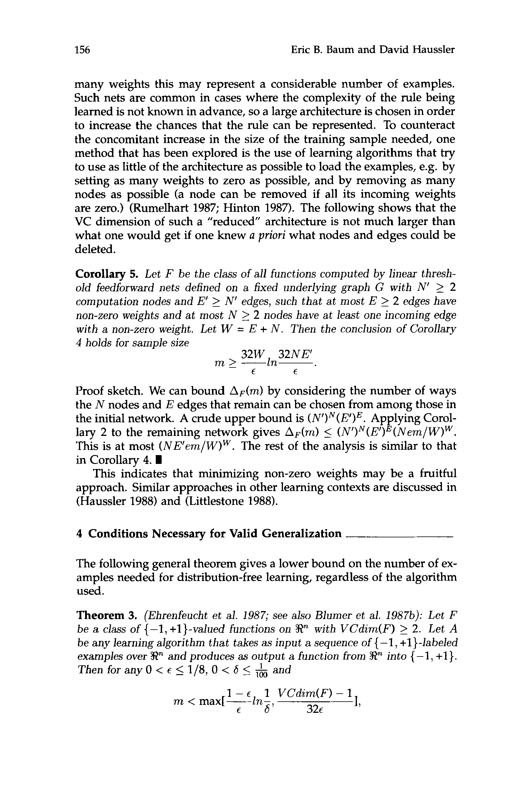
is easily verified that for N 2 2 and m = 2Wlog(eN), ( N e m / metro < 2". Hence this is an upper bound on VCdim(F). I Using VC dimension bounds given in (Wenocur and Dudley 19811, related corollaries can be obtained for nets that use spherical and other types of polynomial threshold functions. These bounds can be used in the following. Theorem 2. (Vapnik 1982) (see Blumer et al. 1987b; Theorem A3.3): Let F 0 < y 5 1, 0 < E , 6 < 1. Let S be a random be a class o f function2 on %In, sequence o f m examples drawn independently according to the distribution D. The probability that there exists a function in F that disagrees with at o f the examples in S and yet has error greater than most a fraction (1 - 7 ) ~ t (w.r.t. D ) is less than 8AF(2m)e-72e"i4. From Corollary 2 and Theorem 3, we get: l D o w n o a d e d f r o m h t t p : / / d i r e c t . m i t . 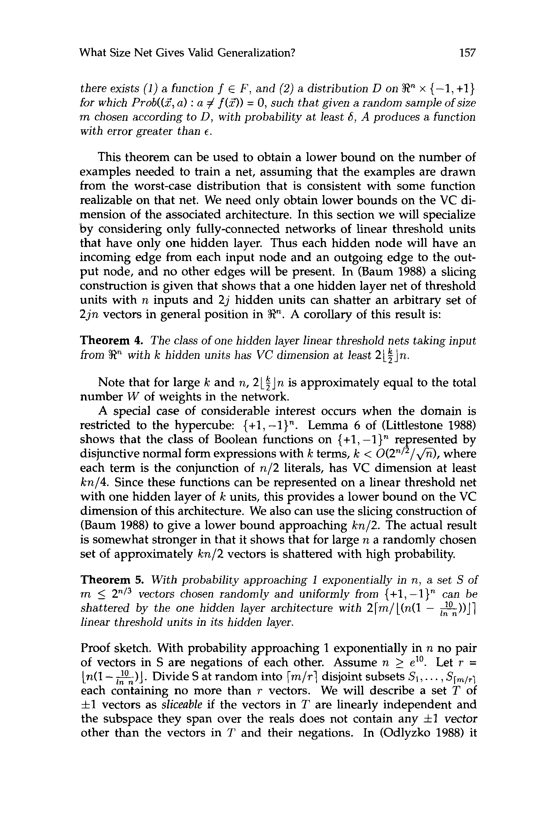Corollary 4. Given a fixed graph G with E edges and N linear threshold units (i.e. W = E + N weights), fixed 0 < E 5 112, and m random training examples, where 32W 32N m 2 -En-, E t i f one can find a choice of weights so that at least a fraction 1 - €12 o f the m training examples are correctly loaded, then one has confidence at least 1 - 8e-1.sw that the net will correctly classify all but a fraction E o f future examples drawn from the same distribution. For 64W 64N m 2 -En-, E E the confidence is at least 1 - 8e-em/32 Proof. Let y = 112 and apply Theorem 3, using the bound on AF(m) given in Corollary 2. This shows that the probability that there exists a choice of the weights that defines a function with error greater than E that is consistent with at least a fraction 1 - €12 of the training examples is at most 8( 2 N em/ W ) w e-'"/16. When m = ?En?, for N 2 2 and t 5 112. When m 2 ?En?, 8(2Nem/W)we-'m/'6 < - 8e-cm/32. I this is 8 ( 2 e & E n y ) W , which is less than 8e-1.5w ( 2 N e m / W ) w 5 efm/32, so The constant 32 is likely an overestimate. No serious attempt has been made to minimize it. Further, we do not know if the log term is unavoidable. Nevertheless, even without these terms, for nets with 2We assume some measurability conditions on the class F. See (Pollard 1984; Blumer et al. 198%) for details. / e d u n e c o a r t i c e - p d / l f / / / / / 1 1 1 5 1 8 1 1 8 1 7 n e c o 1 9 8 9 1 1 1 5 1 p d . . . . . f b y g u e s t t o n 0 7 S e p e m b e r 2 0 2 3 156 Eric B. Baum and David Haussler many weights this may represent a considerable number of examples. Such nets are common in cases where the complexity of the rule being learned is not known in advance, so a large architecture is chosen in order to increase the chances that the rule can be represented. To counteract the concomitant increase in the size of the training sample needed, one method that has been explored is the use of learning algorithms that try to use as little of the architecture as possible to load the examples, e.g. by setting as many weights to zero as possible, and by removing as many nodes as possible (a node can be removed if all its incoming weights are zero.) (Rumelhart 1987; Hinton 1987). The following shows that the VC dimension of such a ”reduced architecture is not much larger than what one would get if one knew a priori what nodes and edges could be deleted. 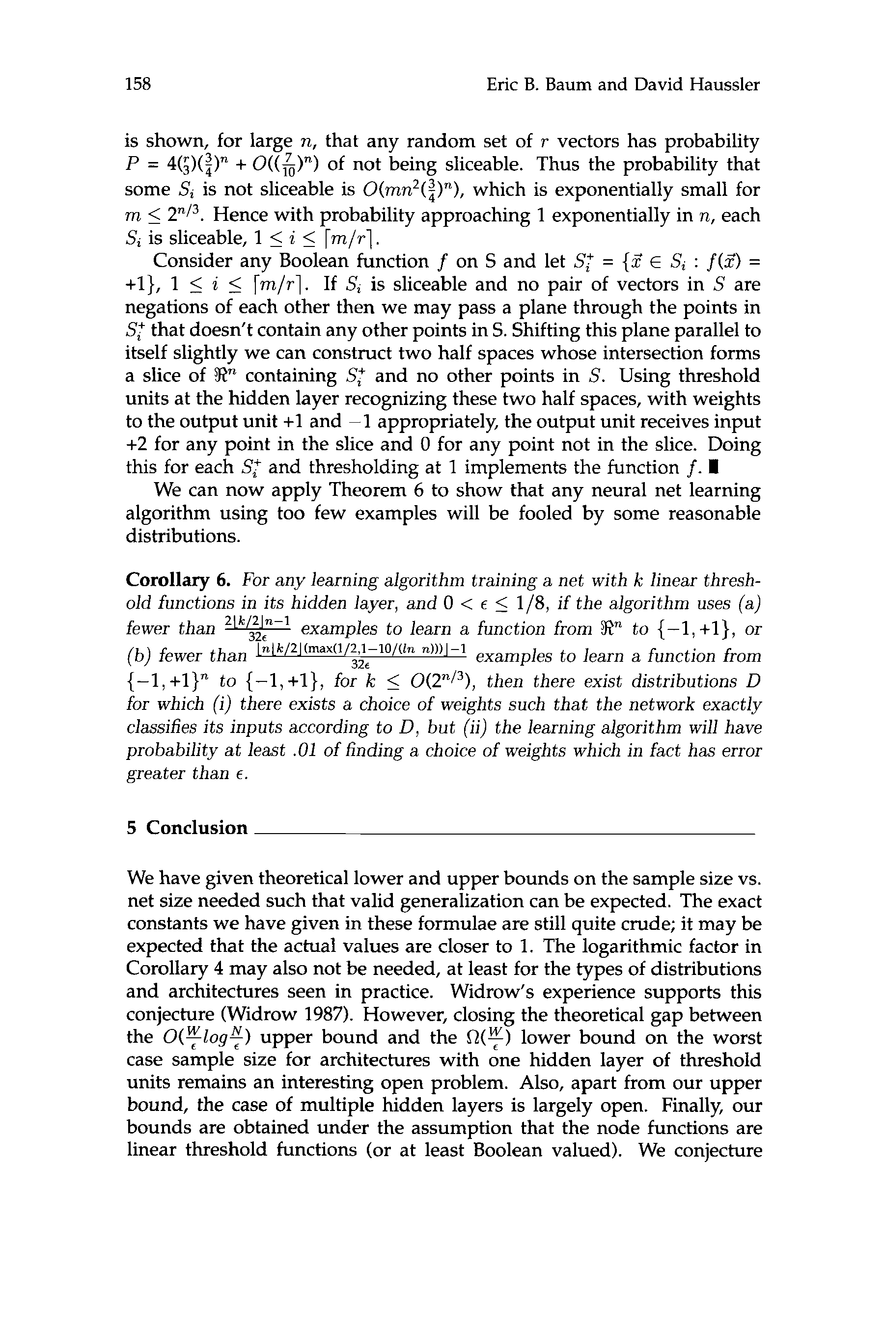Corollary 5. Let F be the class of all functions computed by linear thresh- old feedforward nets defined on a fixed underlying graph G with N‘ > 2
computation nodes and E’ 2 N’ edges, such that at most E 2 2 edges have
non-zero weights and a t most N 2 2 nodes have at least one incoming edge
with a non-zero weight. Let W = E + norte . Then the conclusion of Corollary
4 holds for sample size

32W.
metro 2 —In-.

mi

32NE‘

mi

Proof sketch. We can bound A,(metro) by considering the number of ways
the N nodes and E edges that remain can be chosen from among those in
the initial network. A crude upper bound is (N’)norte(E’)mi. Applying Corol-
lary 2 to the remaining network gives A,(metro) 5 (N’)norte(E’)mi(Nern/W)W..
This is at most (NE’em/W)W.. The rest of the analysis is similar to that
in Corollary 4. I

This indicates that minimizing non-zero weights may be a fruitful
acercarse. Similar approaches in other learning contexts are discussed in
(Haussler 1988) y (Littlestone 1988).

4 Conditions Necessary for Valid Generalization

The following general theorem gives a lower bound on the number of ex-
amples needed for distribution-free learning, regardless of the algorithm
usado.

Teorema 3. (Ehrenfeucht et al. 1987; see also BJumer et aJ. 1987b): Let F
be a class of {-1, +yo}-valued functions on Xn with VCdzm(F) 2 2. Let A
be any learning algorithm that takes as input a sequence of {-1, +I}-labeled
examples over W and produces as output a function from Xn into {-1, +yo}.
Then for any 0 < E 5 1/8, 0 < 6 5 6 and l D o w n o a d e d f r o m h t t p : / / d i r e c t . m i t . / e d u n e c o a r t i c e - p d / l f / / / / / 1 1 1 5 1 8 1 1 8 1 7 n e c o 1 9 8 9 1 1 1 5 1 p d . . . . . f b y g u e s t t o n 0 7 S e p e m b e r 2 0 2 3 I - E 1 VCdim(F)-l m < max[---ln-, € 6 326 I, What Size Net Gives Valid Generalization? 157 there exists (1) a function f E F , and (2) a distribution D on X n x {-1, +1} for which Prob((2, a ) : a # f (2)) = 0 , such that given a random sample of size m chosen according to D , with probability at least 6, A produces a function with error greater than E . This theorem can be used to obtain a lower bound on the number of examples needed to train a net, assuming that the examples are drawn from the worst-case distribution that is consistent with some function realizable on that net. We need only obtain lower bounds on the VC di- mension of the associated architecture. In this section we will specialize by considering only fully-connected networks of linear threshold units that have only one hidden layer. Thus each hidden node will have an incoming edge from each input node and an outgoing edge to the out- put node, and no other edges will be present. In (Baum 1988) a slicing construction is given that shows that a one hidden layer net of threshold units with n inputs and 2 j hidden units can shatter an arbitrary set of 2jn vectors in general position in %In. A coroIlary of this result is: Theorem 4. The class of one hidden layer linear threshold nets taking input from Xn with k hidden units has VC dimension at least 21$]n. Note that for large k and n, 2LSJn is approximately equal to the total number W of weights in the network. A special case of considerable interest occurs when the domain is restricted to the hypercube: {+1, -1)". Lemma 6 of (Littlestone 1988) represented by shows that the class of Boolean functions on {+l, disjunctive normal form expressions with k terms, k < O(Z"/'/fl, where each term is the conjunction of n/2 literals, has VC dimension at least kn/4. Since these functions can be represented on a linear threshold net with one hidden layer of k units, this provides a lower bound on the VC dimension of this architecture. We also can use the slicing construction of (Baum 1988) to give a lower bound approaching kn/2. The actual result is somewhat stronger in that it shows that for large n a randomly chosen set of approximately kn/2 vectors is shattered with high probability. Theorem 5. With probability approaching 1 exponentially in n, a set S of m 5 P I 3 vectors chosen randomly and uniformly from {+l,-l}n can be shattered by the one hidden layer architecture with 2[m/L(n(l - $)-))]I linear threshold units in its hidden layer. Proof sketch. With probability approaching 1 exponentially in n no pair of vectors in S are negations of each other. Assume n 2 e". Let r = Ln(1- &I]. Divide S at random into [ m / ~ l disjoint subsets St,. . . , Srm/rl each containing no more than T vectors. We will describe a set T of 3 ~ 1 vectors as sliceable if the vectors in T are linearly independent and the subspace they span over the reals does not contain any i l vector other than the vectors in T and their negations. In (Odlyzko 1988) it l D o w n o a d e d f r o m h t t p : / / d i r e c t . m i t . / e d u n e c o a r t i c e - p d / l f / / / / / 1 1 1 5 1 8 1 1 8 1 7 n e c o 1 9 8 9 1 1 1 5 1 p d . . . . . f b y g u e s t t o n 0 7 S e p e m b e r 2 0 2 3 158 Eric B. Baum and David Haussler is shown, for large n, that any random set of r vectors has probability P = 4($)(:)" + O((&)") of not being sliceable. Thus the probability that some S, is not sliceable is O(rnn2(:)"), which is exponentially small for rn 5 2n/3. Hence with probability approaching 1 exponentially in R, each S, is sliceable, 1 5 i 5 [rn/rl. Consider any Boolean function f on S and let Sl = ( 2 E S, : f(2) = +1}, 1 5 i 5 [m/r1. If S, is sliceable and no pair of vectors in S are negations of each other then we may pass a plane through the points in S,+ that doesn't contain any other points in S. Shifting this plane parallel to itself slightly we can construct two half spaces whose intersection forms a slice of !R" containing S,+ and no other points in S. Using threshold units at the hidden layer recognizing these two half spaces, with weights to the output unit +1 and -1 appropriately, the output unit receives input +2 for any point in the slice and 0 for any point not in the slice. Doing this for each 5': and thresholding at 1 implements the function f. I We can now apply Theorem 6 to show that any neural net learning algorithm using too few examples will be fooled by some reasonable distributions. Corollary 6. For any learning algorithm training a net with k linear thresh- old functions in its hidden layer, and 0 < E < 118, if the algorithm uses (a) examples to learn a function from F' to {-l,+l}, or fewer than (b) fewer than Lnlk/Z] (max(l/2,1-10/(ln examples to learn a function from {-l,+l}" to {-l,+l}, for k 5 O(2"I3), then there exist distributions D for which (i) there exists a choice of weights such that the network exactly classifies its inputs according to D , but (ii) the learning algorithm will have probability a t least .01 of finding a choice of weights which in fact has error greater than E . "I))] -1 326 5 Conclusion We have given theoretical lower and upper bounds on the sample size vs. net size needed such that valid generalization can be expected. The exact constants we have given in these formulae are still quite crude; it may be expected that the actual values are closer to 1. The logarithmic factor in Corollary 4 may also not be needed, at least for the types of distributions and architectures seen in practice. Widrow's experience supports this conjecture (Widrow 1987). However, closing the theoretical gap between the O(5log:) upper bound and the R ( 7 ) lower bound on the worst case sample size for architectures with one hidden layer of threshold units remains an interesting open problem. Also, apart from our upper bound, the case of multiple hidden layers is largely open. Finally, our bounds are obtained under the assumption that the node functions are linear threshold functions (or at least Boolean valued). We conjecture l D o w n o a d e d f r o m h t t p : / / d i r e c t . m i t . / e d u n e c o a r t i c e - p d / l f / / / / / 1 1 1 5 1 8 1 1 8 1 7 n e c o 1 9 8 9 1 1 1 5 1 p d . . . . . f b y g u e s t t o n 0 7 S e p e m b e r 2 0 2 3 What Size Net Gives Valid Generalization? 159 that similar bounds also hold for classes of real valued functions such as sigmoid functions, and hope shortly to establish this. Acknowledgments We would like to thank Ron Rivest for suggestions on improving the bounds given in Corollaries 4 and 5 in a n earlier draft of this paper, and Nick Littlestone for many helpful comments. The research of E. Baum was performed by the Jet Propulsion Laboratory, California Institute of Technology, as part of its Innovative Space Technology Center, which is sponsored by the Strategic Defense Initiative Organization/Innovative Science and Technology through an agreement with the National Aero- nautics and Space Administration (NASA). D. Haussler gratefully ac- knowledges the support of ONR grant N00014-86-K-0454. Part of this work was done while E. Baum was visiting UC Santa Cruz. l D o w n o a d e d f r o m h t t p : / / d i r e c t . m i t . References Baum, E.B. 1988. On the Capabilities of Multilayer Perceptrons. J. of Complexity, in press. Blumer, A., A. Ehrenfeucht, D. Haussler, and M. Warmuth. 1987a. Occam’s Razor. lnf. Proc. Let. 24, 377-380. . 1987b. Learnability and the Vapnik-Ckervonenkis Dimension. University of California-Santa Cruz Technical Report UCSC-CRL-87-20 and I. ACM, to appear. Cover, T. 1965. Geometrical and Statistical Properties of Systems of Linear Inequalities with Applications to Pattern Recognition. IEEE Trans. Elect. Comp. V14,326-334. Devroye, L. 1988. Automatic Pattern Recognition, a Study of the Probability of Error. I E E E Trans. PAMI V10:N4, 530-543. Denker, J., D. Schwartz, B. Wittner, S. Solla, J. Hopfield, R. Howard, and L. Jackel. 1987. Automatic Learning, Rule Extraction, and Generalization. Complex Systems 1, 877-922. Duda, R. and P. Hart. 1973. Pattern Classification and Scene Analysis. New York: Wiley. Ehrenfeucht, A., D. Haussler, M. Kearns, and L. Valiant. 1987. A General Lower Bound on the Number of Examples Needed for Learning. University of California-Santa Cruz Technical Report UCSC-CRL-87-26 and Information and Computation, to appear. Haussler, D. 1988. Quantifying Inductive Bias: A1 Learning Algorithms and Valiant’s Learning Framework. Artificial Intelligence 36, 177-221. Hinton, G. 1987. Connectionist Learning Procedures. Artificial Intelligence, to appear. Littlestone, N. 1988. Learning Quickly when Irrelevant Attributes Abound: a new linear threshold algorithm. Machine Learning V2, 285-318. / e d u n e c o a r t i c e - p d / l f / / / / / 1 1 1 5 1 8 1 1 8 1 7 n e c o 1 9 8 9 1 1 1 5 1 p d . . . . . f b y g u e s t t o n 0 7 S e p e m b e r 2 0 2 3 160 Eric B. Baum and David Haussler Odlyzko, A. 1988. On Subspaces Spanned by Random Selections of f l Vectors. J. Comb. Th. A V47:N1,124-133. Pollard, D. 1984. Convergence of stochastic processes. New York: Springer-Veriag. Qian, N. and T.J. Sejnowski. 1988. Predicting the Secondary Structure of Glob- ular Protein using Neural Networks. J. Molec. Bid. 202, 865-884. Rumelhart, D. 1987. Personal communication. Sauer, N. 1972. On the Density of Families of Sets. J. Comb. 7%. A V13,145-147. Sejnowski, T.J. and C.R. Rosenberg. 1987. NET Talk a Parallel Network that Learns to Read Aloud. Complex Systems 1, 145-168. Tesauro, G. and T.J. Sejnowski. 1988. A 'Neural' Network that Learns to Play Backgammon. In: Neural Information Processing Systems, ed. D.Z. Ander- son, AIP, NY, 794-803. Valiant, L.G. 1984. A Theory of the Learnable. Comm. ACM V27 N11,1134-1142. Vapnik, V.N. and A.Ya. Chervonenkis. 1971. On the Uniform Convergence of Relative Frequencies of Events to their Probabilities. Th. Prob. and its Applications V12N2, 264-280. Vapnik, V.N. 1982. Estimation of Dependences Based on Empirical Data. New York Springer Verlag. Wenocur, R.S. and R.M. Dudley. 1981. Some Special Vapnik-Chervonenkis Classes. Discrete Math. V33, 313-318. Widrow, B. 1987. ADALINE and MADALINE - 1963, Plenary Speech, Vol I: Proc. IEEE Zst Int. Conf. on Neural Networks, San Diego, CA, 143-158. Received 5 September; accepted 26 September 1988. l D o w n o a d e d f r o m h t t p : / / d i r e c t . m i t . / e d u n e c o a r t i c e - p d / l f / / / / / 1 1 1 5 1 8 1 1 8 1 7 n e c o 1 9 8 9 1 1 1 5 1 p d . . . . . f b y g u e s t t o n 0 7 S e p e m b e r 2 0 2 3

Descargar PDF