RESEARCH PAPER
RS-SVM Machine Learning Approach Driven by Case
Data for Selecting Urban Drainage Network Restoration
Scheme
Li Jiang1, Zheng Geng1, Dongxiao Gu1†, Shuai Guo2, Rongmin Huang3, Haoke Cheng3, Kaixuan Zhu4
1School of Management, Hefei University of Technology, Hefei 230002, China
2College of Civil Engineering, Hefei University of Technology, Hefei 230002, China
3Yangtze Ecology and Environment Co.,Ltd., Wuhan 430062, China
4Luddy School of Intelligent System and Engineering, Indianan university, Bloomington, Indiana 47404, USA
Keywords: Drainage pipe network; Machine learning; Rough set; Multilevel SVM; Restoration scheme
Citation: Jiang, L., Geng, Z., Gu, D.X. et al.: RS-SVM machine learning approach driven by case data for selecting urban drainage
network restoration scheme. Data Intelligence 5(2), 413-437 (2023). doi: 10.1162/dint_a_00208
Submitted: Janurary 15, 2023; Revised: Febbraio 14, 2023; Accepted: Marzo 10, 2023
ABSTRACT
Urban drainage pipe network is the backbone of urban drainage, flood control and water pollution
prevention, and is also an essential symbol to measure the level of urban modernization. A large number of
underground drainage pipe networks in aged urban areas have been laid for a long time and have reached
or practically reached the service age. The repair of drainage pipe networks has attracted extensive attention
from all walks of life. Since the Ministry of ecological environment and the national development and Reform
Commission jointly issued the action plan for the Yangtze River Protection and restoration in 2019, various
provinces in the Yangtze River Basin, such as Anhui, Jiangxi and Hunan, have extensively carried out PPP
projects for urban pipeline restoration, in order to improve the quality and efficiency of sewage treatment.
Based on the management practice of urban pipe network restoration project in Wuhu City, Anhui Province,
this paper analyzes the problems of lengthy construction period and repeated operation caused by the
mismatch between the design schedule of the restoration scheme and the construction schedule of the pipe
network restoration in the existing project management mode, and proposes a model of urban drainage pipe
network restoration scheme selection based on the improved support vector machine. The validity and
feasibility of the model are analyzed and verified by collecting the data in the project practice. The research
results show that the model has a favorable effect on the selection of urban drainage pipeline restoration
†
Corresponding author: DongXiao Gu (e-mail: dongxiaogu@yeah.net; ORCID: 0000-0003-3557-009X).
© 2023 Chinese Academy of Sciences. Published under a Creative Commons Attribution 4.0 Internazionale (CC BY 4.0)
licenza.
l
D
o
w
N
o
UN
D
e
D
F
R
o
M
H
T
T
P
:
/
/
D
io
R
e
C
T
.
M
io
T
.
e
D
tu
D
N
/
io
T
/
l
UN
R
T
io
C
e
–
P
D
F
/
/
/
/
5
2
4
1
3
2
0
8
9
8
0
9
D
N
_
UN
_
0
0
2
0
8
P
D
/
.
T
io
F
B
sì
G
tu
e
S
T
T
o
N
0
7
S
e
P
e
M
B
e
R
2
0
2
3
RS-SVM Machine Learning Approach Driven by Case Data for Selecting Urban Drainage
Network Restoration Scheme
schemes, and its accuracy can reach 90%. The research results can provide method guidance and technical
support for the rapid decision-making of urban drainage pipeline restoration projects.
1. INTRODUCTION
With the rapid urbanization, the short board of urban drainage pipe network construction is showing up
daily. Various structural and functional defects of the drainage pipe network caused by aging easily cause
problems such as urban waterlogging, sewage overflow, and ground subsidence [1]. Therefore, completing
the urban drainage pipe network detection and repair is critical for realizing city sewage quality and
efficiency, which helps promote the development of high-quality urban governance. Tuttavia, the urban
drainage pipe network has long miles, complicated structure, uncertainty factors, and extensive range,
which significantly influences residents’ living environment and urban traffic [2]. Così, how to determine
the drainage pipe network’s status and performance, design reasonable repair scheme rapidly, shorten the
whole pipeline repair project period, and reduce the project construction according to its testing results
can greatly affect the social environment and sustainable development.
In recent years, the introduction of pipe network performance evaluation technology has made the best
solution for pipe repair, which has become a research hot spot among domestic and foreign scholars and
experts. The existing research mainly uses qualitative and quantitative research methods to establish the
prediction model of pipe network performance indicators and formulate maintenance plans. Tuttavia, UN
difficult problem remains, which is the low efficiency of the decision making. Using machine learning-
related technologies in mining case history, the literature that studies the quick decisions for fixing urban
drainage pipe networks is scant.
Così, this research put forward RS-SVM machine learning approach driven by case data for selecting
urban drainage network restoration scheme. The main contribution of this study is threefold. Primo, we
combine the attribute reduction based on RS technology [3] and the SVM technology [4] to give full play
to their technological advantages. The minimalist data set of the excellent classification characteristics is
used as the input of the SVM. Secondo, we propose an RS-SVM model for selecting an urban drainage pipe
network repair scheme. The basic idea is to collect history data set from urban pipeline repairing project
management practice for a pipeline, use RS theory to reduce the sample’s attributes, use the indirect method
combining two classifiers to construct a multi-level SVM scheme selection model, and then use the built
model for scheme selection of the test sample to solve the matching analysis. Finalmente, we select Wuhu’s
drainage pipeline repair engineering case data for big data analysis in Anhui Province. The effectiveness of
the proposed model and method is verified. This study provides decision support for the quick selection of
drainage pipeline repair schemes and has a certain application value.
2. RELATED WORKS
As for the technology on predicting the state of pipe network and developing repair strategies, Altarabsheh
A et al. [5] used the Markov model to predict pipeline networks in the future and choose the most
414
Data Intelligence
l
D
o
w
N
o
UN
D
e
D
F
R
o
M
H
T
T
P
:
/
/
D
io
R
e
C
T
.
M
io
T
.
e
D
tu
D
N
/
io
T
/
l
UN
R
T
io
C
e
–
P
D
F
/
/
/
/
5
2
4
1
3
2
0
8
9
8
0
9
D
N
_
UN
_
0
0
2
0
8
P
D
/
T
.
io
F
B
sì
G
tu
e
S
T
T
o
N
0
7
S
e
P
e
M
B
e
R
2
0
2
3
RS-SVM Machine Learning Approach Driven by Case Data for Selecting Urban Drainage
Network Restoration Scheme
appropriate operational plan by GA, according to the whole life cycle of a sewage pipe network, considering
the construction cost, operation cost, and expected benefits. Hernández N et al. [6] used the differential
evolution method as an optimization tool for hyperparameter combination and combined it with the SVM
model for two different management objectives (network and pipe levels). This model was applied to
Colombia’s main cities of Bogotá and Medellin, resulting in a less than 6% deviation in the prediction of
structural conditions in both cities at a network level. Wang Y J et al. [7] proposed an XGBoost-based MICC
model with the benefits of hyperparameters autooptimization. Yu A L et al. [8] put forward a method to
carry out the five directions of research for the drainage pipeline repair scheme. Intelligent decision provides
the basis. To predict the future performance of trenchless rehabilitations, Ibrahim B et al. [9] presented
condition prediction models for the chemical grouting rehabilitation of pipelines and manholes in the city
of Laval, Quebec, Canada. Bakry I et al. [10] presented condition prediction models for CIPP rehabilitation
of sewer mains, and the models can predict the structural and operational conditions of CIPP rehabilitation
on the basis of basic input, such as pipe material, and rehabilitation type and date.
As for the technology on development of decision support tools for drainage network repair, Cai X T et
al. [11] proposed a sensitivity-based adaptive procedure (SAP), which can be integrated with optimization
algorithms. SAP was integrated with non-dominated sorting genetic algorithm II (NSGA-II) and multiple
objective particle swarm optimization (MOPSO) metodi. Ulrich A et al. [12] studied a novel solution
combining both approaches (pipes and tanks) and proposed a decision support system based on the NSGA-II
for the rehabilitation of urban drainage networks through the substitution of pipes and the installation of
storage tanks. Debères P et al. [13] used multiple criteria to locate the repair section and made a repair
plan according to the pipeline inspection report and the economic, social, and environmental indicators.
Ramos-Salgado et al. [14] developed a decision support system (DSS) to help water utilities design
intervention programs for hydraulic infrastructures. Chen S B et al. [15] summarized the characteristics,
causes, and evolution mechanism of typical defect types of coastal urban drainage network, which can
provide technical guidance for the evaluation and repair of drainage network in this area or similar cities.
Based on the investigation of the current situation of the existing underground drainage network in a certain
area of Chongqing, Liu W et al. [16] used the AHP and entropy weight method to study the urban drainage
pipe network risk rating and provide decision support for pipeline repair plan design. In view of the urban
drainage pipe network deterioration, Wang J L et al. [17] used AHP and fuzzy comprehensive evaluation
methods to research the urban drainage pipe network status and operational efficiency to provide decision
support for drainage pipe network maintenance and repair plan.
This study is inspired by Xie B et al. [18] but different from the previous works that focused on designating
remediation solutions based on current drainage inspection results but does not sufficiently explore the
value of historical cases to solve this current problem. The choice of an urban drainage pipeline repair plan
belongs to the category of multiple attribute decision making [19]. For multiple attribute decision-making
problems, policymakers tend to be objective in formulating the optimal alternatives [20]. Support vector
machine (SVM) is established on VC dimension theory and structural risk minimization principle based on
machine learning methods [21]. It has better properties, especially in quickly setting the optimal alternative
Data Intelligence
415
l
D
o
w
N
o
UN
D
e
D
F
R
o
M
H
T
T
P
:
/
/
D
io
R
e
C
T
.
M
io
T
.
e
D
tu
D
N
/
io
T
/
l
UN
R
T
io
C
e
–
P
D
F
/
/
/
/
5
2
4
1
3
2
0
8
9
8
0
9
D
N
_
UN
_
0
0
2
0
8
P
D
T
.
/
io
F
B
sì
G
tu
e
S
T
T
o
N
0
7
S
e
P
e
M
B
e
R
2
0
2
3
RS-SVM Machine Learning Approach Driven by Case Data for Selecting Urban Drainage
Network Restoration Scheme
for current cases based on multi-attribute case history data [22]. As the SVM’s input, the case history data
sets frequently have redundant attributes [23]. Redundant attributes can increase the complexity of SVM
training, extend the SVM training time, and reduce the SVM decision efficiency. A rough set (RS) deals with
the uncertainty problem of mathematical tools [24]. RS attribute reduction algorithm can effectively handle
attribute redundancy; it reduces redundant attributes that interfere with the SVM. Così, on the basis of the
combination of rough set and SVM technology, we propose an RS-SVM model for selecting an urban
drainage network restoration scheme in this study.
3. METHODOLOGY
The detailed process of combining RS and SVM to select an urban drainage pipe network repair scheme
consists of four components. The structure of which is shown in Figure 1, and the role of each component
is as follows:
• Collecting historical data sets and then standardizing them.
• Using the RS attribute reduction algorithm to reduce the redundant attributes contained in the data
set.
• Training the model of multi-level SVM classification.
• Using the trained model to match the new detection results.
l
D
o
w
N
o
UN
D
e
D
F
R
o
M
H
T
T
P
:
/
/
D
io
R
e
C
T
.
M
io
T
.
e
D
tu
D
N
/
io
T
/
l
UN
R
T
io
C
e
–
P
D
F
/
/
/
/
5
2
4
1
3
2
0
8
9
8
0
9
D
N
_
UN
_
0
0
2
0
8
P
D
.
T
/
io
F
B
sì
G
tu
e
S
T
T
o
N
0
7
S
e
P
e
M
B
e
R
2
0
2
3
Figura 1. Detailed process of combining RS and SVM to select an urban drainage pipe network repair
scheme.
The related parameters described in the model are as follows: {Z1, Z2,…, Zi,…, Zm} are the historical data
sets of drainage pipeline repair projects. The target case denoted by Z0 is the current case reflecting the
416
Data Intelligence
RS-SVM Machine Learning Approach Driven by Case Data for Selecting Urban Drainage
Network Restoration Scheme
P, C2
P,…, Cj
P,…, Cn
P} is the attribute set of drainage pipe network detection
need for a repair scheme. {C1
p value corresponding to
risultati. (a01, a02,…, a0j,…, a0n) is the attribute value vector of Z0, where a0j is the Cj
Z0. In this study, the drainage pipe network detection properties are divided into two types, numeric and
symbols. Per esempio, the length, diameter, various defects, and quantity of the pipes belong to numeric
dati. The material of the pipes belongs to symbol data. {S1,S2,…,Sk,…,Sg} is the history solution set of
drainage pipeline repair projects. According to the characteristics of the urban pipeline repair project, we
presume that a solution may apply to multiple cases, with each case only a final implementation scheme.
3.1 Standardizing
To eliminate the influence of the dimension, we need to standardize the data set. Symbol variables are
denoted by {Fi|iT}, where T equals {1, 2, 3, …, T}. Così, we set the symbol sequence within the specified
symbol in advance. The sequence number of the Sign Fi is seq(Fi), where FiF, seq(Fi)T. Standardizing the
symbolic variables uses Equation (1):
=
‘
F
io
(F )io
seq
T
(1)
We use the normal method to standardize some numeric variables. This method is suitable for indicators
with a nonzero-range. The standardized variable values are between 0 E 1. Standardizing the symbolic
variables uses Equation (2):
=
X
‘
io
X
io
max(
X
– min(
X
)
) – min(
io
io
X
io
)
(2)
3.2 RS Attributes Reduction
Selecting as many attributes that have a greater impact on the scheme as possible can avoid missing
crucial ones. If there are a large number of attributes, the complexity of the model inevitably increases,
and the prediction performance is reduced, supposing all attributes are input into the SVM model. Some
attributes have little influence on the selection of repair schemes for urban drainage networks, and the
repair schemes are determined to some extent by a few key attributes that best reflect the characteristics
of the categories [25]. Therefore, attribute reduction is conducive to improving the prediction accuracy and
efficiency of the SVM model. In light of the influence of the definition of attribute importance and reduction
rules, the result of attribute reduction is often not unique, and finding a minimum reduction has been
proven to be an NP-hard problem [26]. The general method to solve this problem is to find the optimal or
suboptimal reduction by heuristic search method [27]. Così, we propose the attribute reduction algorithm
based on attribute similarity. The basic flow of the algorithm is as follows:
Step 1: All conditional attributes are reduced using discernible attribute matrix.
In rough set theory, tuples S=(U, UN, V, F ) are defined as information systems, where U is a discussion
domain of A, A=C∪D is an attribute set, C represents conditional attributes, and D represents target
attributes. In the information system S, the differentiation determined by RA is: A=U/RA={Ki: i≤l }, and fl
Data Intelligence
417
l
D
o
w
N
o
UN
D
e
D
F
R
o
M
H
T
T
P
:
/
/
D
io
R
e
C
T
.
M
io
T
.
e
D
tu
D
N
/
io
T
/
l
UN
R
T
io
C
e
–
P
D
F
/
/
/
/
5
2
4
1
3
2
0
8
9
8
0
9
D
N
_
UN
_
0
0
2
0
8
P
D
T
/
.
io
F
B
sì
G
tu
e
S
T
T
o
N
0
7
S
e
P
e
M
B
e
R
2
0
2
3
RS-SVM Machine Learning Approach Driven by Case Data for Selecting Urban Drainage
Network Restoration Scheme
(Ki) is used to represent the value of attribute cl with respect to the object in Ki, called I(Ki, Kj) ( Equazione
(3)). It is the discernable attribute matrix of Ki and Kj, and the main diagonal element of I is the empty set.
I K K
,
(
io
j
)
=
The identification equation is as follows:
M
∈
c A f K
{
:
(
l
l
≠
)
io
f K
(
l
j
)}
= ∧ ∨
(
≠
io
j
D c c
(
io
,
))
j
(3)
(4)
All attributes of the information system can be reduced using Equation (4). Per esempio, in the information
system shown in Table 1, {c1, c2, c3, c4} is the conditional attribute and D is the decision attribute.
Tavolo 1. Information system.
code
Z1
Z2
Z3
Z4
c1
2
3
2
1
c2
1
2
1
1
c3
3
1
3
4
D
0
1
0
3
code
Z5
Z6
Z7
Z8
c1
1
1
1
1
c2
1
1
2
2
c3
2
4
3
3
D
4
3
2
2
According to Table 1, the samples with the same attribute value are merged to obtain the simplified
information system shown in Table 2.
code
K1 = {Z1,Z3}
K2 = {Z2}
K3 = {Z7,Z8}
K4 = {Z4,Z6}
K5={Z5}
Tavolo 2. Simplifi ed information system.
c1
2
3
1
1
1
c2
1
2
2
1
1
c3
3
1
3
4
2
D
0
1
2
3
4
From Table 2 and Formula (3), the discernable attribute matrix I shown in Table 3 is obtained.
Tavolo 3. Discernible attribute matrix I.
IO
K1
K2
K3
K4
K5
K1
∅
{c1,c2,c3}
{c1,c2}
{c1,c3}
{c1,c3}
K2
{c1,c2,c3}
∅
{c1,c3}
{c1,c2,c3}
{c1,c2,c3}
K3
{c1,c2}
{c1,c3}
∅
{c2,c3}
{c2,c3}
K4
{c1,c3}
{c1,c2,c3}
{c2,c3}
∅
{c3}
K5
{c1,c3}
{c1,c2,c3}
{c2,c3}
{c3}
∅
In Table 3, according to the discernable attribute matrix I and Equation (4), all the reductions of the
information system are obtained as G1={c1, c3} and G2={c2, c3}.
418
Data Intelligence
l
D
o
w
N
o
UN
D
e
D
F
R
o
M
H
T
T
P
:
/
/
D
io
R
e
C
T
.
M
io
T
.
e
D
tu
D
N
/
io
T
/
l
UN
R
T
io
C
e
–
P
D
F
/
/
/
/
5
2
4
1
3
2
0
8
9
8
0
9
D
N
_
UN
_
0
0
2
0
8
P
D
.
T
/
io
F
B
sì
G
tu
e
S
T
T
o
N
0
7
S
e
P
e
M
B
e
R
2
0
2
3
RS-SVM Machine Learning Approach Driven by Case Data for Selecting Urban Drainage
Network Restoration Scheme
Step 2: The core of the information system should be found.
Equazione (5) is used to find the core of the information system, Dove {Gi: i≤l} represents all reductions
of the information system.
core()
l
= ∩
G
io
i =
1
(5)
According to the result of step 1 and Eq uation (5), the core of the information system can be obtained
as core()=G1
∩G2={c1, c3}∩{c2, c3}={c3}.
Step 3: The similarity of relatively necessary attributes is calculated with respect to decision attribute D.
If the core is not empty, any reduction contains the core. So the properties in the core are absolutely
necessary properties. Equazione (6) is used to represent the set of relatively necessary attributes that appear
in some reductions.
rna()
=
l
l
−∪
G
io
∩
G
io
=
io
1
io
=
1
(6)
According to the result of Step 2 and Equation (6), the relatively necessary attributes of the information
system can be obtained: rna()={c1, c3}∪{c2, c3}-{c1, c3}∩{c2, c3}={c1, c2}.
Step 4: The similarity between each relatively necessary attribute and decision attribute is gradually
added to the core in order from high to low to form set R until R satisfies the indistinguishable relation:
IND (R) = IND(C). Therefore, R is the relative minimum.
The similarity between conditional attribute {C} and decision attribute D is calculated by Equation (7).
{ }
S( C ,D)
=
∪
{ }
IND(D c )
⋅
{ }
IND( C )
IND(D)
(7)
According to Table 1, S(c1,D) and S(c2,D) are calculated by the following equation:
S(C ,D)
1
=
S(C ,D)
2
=
IND(C )
1
∪
IND(D c )
1
⋅
IND(D)
∪
IND(D c )
2
⋅
IND(D)
IND(C )
2
=
0.683
=
0.642
By virtue of S(c1, D)>S(c2, D), adding the relatively necessary attribute c1 to core() can form the set R1={c1,
c3}. Since IND(R1)=IND(C)=14, the indistinguishable relation is satisfied. Così, {c1, c3} is the relative
minimum for this example.
Data Intelligence
419
l
D
o
w
N
o
UN
D
e
D
F
R
o
M
H
T
T
P
:
/
/
D
io
R
e
C
T
.
M
io
T
.
e
D
tu
D
N
/
io
T
/
l
UN
R
T
io
C
e
–
P
D
F
/
/
/
/
5
2
4
1
3
2
0
8
9
8
0
9
D
N
_
UN
_
0
0
2
0
8
P
D
/
T
.
io
F
B
sì
G
tu
e
S
T
T
o
N
0
7
S
e
P
e
M
B
e
R
2
0
2
3
RS-SVM Machine Learning Approach Driven by Case Data for Selecting Urban Drainage
Network Restoration Scheme
3.3 Selecting Kernel Function
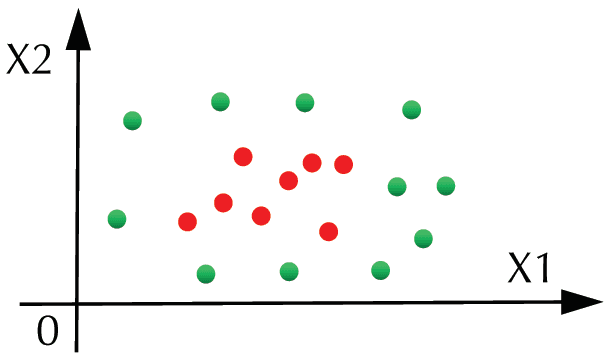
The prerequisite for SVM classification is that the sample space is linearly separable. Tuttavia, IL
complexity of data spatial distribution increases along with the increase of the sample space dimension.
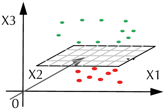
Per esempio, in Figure 2, points are linearly indivisible in a two-dimensional plane. In Figure 3, a kernel
function is adopted to transform the sample dimensionally. The requirement of linear divisibility is satisfied
after the sample set is mapped to a higher-dimensional space. Different kernel functions can be used to
construct and realize different types of nonlinear decision surface learning machines in the input space,
thus generating different support vector algorithms [28]. We select several kernel functions commonly used
in classification problems. Functions (8)-(11) are expressed as follows:
Linear kernel function:
K
,
(
x x
io
j
)
=
⋅
X
T
io
X
j
Poly kernel function:
K
(
x x
,
io
j
)
=
(
X
T
io
⋅
X
j
+
D
)1
,
D
≥
0
RBF kernel function:
K
(
x x
,
io
j
)
=
−
exp γ
(
||
X
io
−
X
j
2
|| )
,
γ
>
0
Sigmoid kernel function:
K
(
x x
,
io
j
)
=
tanh k
(
X
⋅
T
io
X
j
+
c k
,
)
>
0;
C
>
0
(8)
(9)
(10)
(11)
Figura 2. Linearly indivisible points.
Figura 3. Linearly separable points.
l
D
o
w
N
o
UN
D
e
D
F
R
o
M
H
T
T
P
:
/
/
D
io
R
e
C
T
.
M
io
T
.
e
D
tu
D
N
/
io
T
/
l
UN
R
T
io
C
e
–
P
D
F
/
/
/
/
5
2
4
1
3
2
0
8
9
8
0
9
D
N
_
UN
_
0
0
2
0
8
P
D
/
T
.
io
3.4 Training Multi-level SVM Classification Model
3.4.1 Binary Classification Algorithm Based on Historical Cases
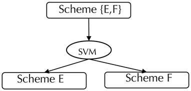
Before building a multi-level SVM classification model, a binary classification model should be built.
Let the scheme set of the sample be {E, F}. In Figure 4, the binary classification problem is to build a binary
classifier that can distinguish schemes E and F through historical cases. The theoretical derivation of the
binary classifier is as follows:
F
B
sì
G
tu
e
S
T
T
o
N
0
7
S
e
P
e
M
B
e
R
2
0
2
3
Figura 4. Work fl ow of binary classifi er.
420
Data Intelligence
RS-SVM Machine Learning Approach Driven by Case Data for Selecting Urban Drainage
Network Restoration Scheme
We set some sample points in the sample space {xi|i=1, 2, 3, …, N}, where xi is the vector corresponding
∈{-1, 1}. IL
to each sample point. yi is the class value corresponding to each sample point, where yi
equations of positive hyperplane H1, negative hyperplane H2 and decision hyperplane H0 are as follows:
⎧
H
1
⎪
⎨
H
0
⎪
H
⎩
2
:
:
:
wx
wx
wx
+ =
B
+ =
B
+ = −
B
+1
0
1
The constrained optimization problem for the maximum value L is written in the following form:
l
max
=
2
w
s t
. . (
⋅
w x
io
+
b y
)
io
≥
1
To facilitate calculation, Equazione (13) is rewritten as
Lar
w
(
,
B
,
λ
,
io
P
io
)
=
T
⋅
w w
2
−
N
∑
=
1
io
The dual problem of Equation (14) is as follows:
λ
io
[(
⋅
w x
+
io
b y
)
io
−
1]
λ
io
≥
0
max(min(
ë
w
,
B
Lar
w
(
,
B
,
λ
,
io
P
io
s t
)) . .
λ ≥
io
0
(12)
(13)
(14)
(15)
Considering the influence of w and b on Lagrange function (15), the following function is constructed.
F
w
(
,
B
)
=
(
T
⋅
w w
2
−
N
∑
=
1
io
λ
io
⋅
w x
((
+
io
b y
)
io
−
1)) ,
λ
io
≥
0
(16)
The argument of function f(w,B) is unconstrained and the function is a convex function about the
argument (w1,w2,w3,…,ws,B), so it has a unique minimum point. Its gradient expression is as follows:
∇
F
w
(
,B)
=
F
F
∂⎡
⎢
⎢
⎢
⎢
⎣
∂
,B)
w
(
∂
w
w
(
,B)
∂
B
⎤
⎥
⎥
⎥
⎥
⎦
=
⎡
w
⎢
⎢
⎢
⎢
⎣
T
−
N
∑
=
io
0
λ
sì
io
io
X
io
N
∑
=
io
0
λ
sì
io
io
⎤
⎥
⎥
⎥
⎥
⎦
λ
io
,
≥
0
Let
f∇
=w
(
,B)
0 ; Equazione (18) can be obtained according to Equation (17):
T
=
N
∑
=
1
io
λ
sì
io
io
X
io
λ
sì
io
io
=
0
⎧
w
⎪
⎪
⎨
⎪
⎪⎩
=
N
io
∑
0
,
≥
λ
io
0
l
D
o
w
N
o
UN
D
e
D
F
R
o
M
H
T
T
P
:
/
/
D
io
R
e
C
T
.
M
io
T
.
e
D
tu
D
N
/
io
T
/
l
UN
R
T
io
C
e
–
P
D
F
/
/
/
/
5
2
4
1
3
2
0
8
9
8
0
9
D
N
_
UN
_
0
0
2
0
8
P
D
.
T
/
io
F
B
sì
G
tu
e
S
T
T
o
N
0
7
S
e
P
e
M
B
e
R
2
0
2
3
(17)
(18)
After substituting Equation (18) into the function and introducing some kernel function, Equazione (15)
can be written as
Data Intelligence
max(
ë
N
∑
=
1
k
λ
k
−
1
2
N
N
∑∑
=
1
io
=
1
j
λλ
io
j
y y K
io
j
(
x x
io
j
s t
)) . .
λ λ
,
io
j
≥
0
(19)
421
RS-SVM Machine Learning Approach Driven by Case Data for Selecting Urban Drainage
Network Restoration Scheme
After solving for
=λ
(
λ λ λ λ
N
3
,…,
,
,
1
2
)T
, we can solve for w* in terms of
N
= ∑w
T
=
1
io
yλ
io
io
X , We just use the
io
support vector xi* in the computation of w*. Positive hyperplane H1: w*x+b*=1. Negative hyperplane H2:
w*x+b*=1. Decision hyperplane H0: w*x+b*=0. After the three hyperplane equations are determined, IL
binary classifier is constructed.
3.4.2 Multi-Classification Method Based on Combinatorial Thinking
The repair schemes of urban drainage pipe networks are diverse, so a single binary classifier cannot
complete the classification of all schemes; combining multiple binary classifiers is necessary. The common
combination methods of binary classification include indirect and direct metho ds [29]. The indirect method
is to construct a series of binary classifiers in a certain way and combine them to achieve multi-class
classificazione. The other combines the parameter solutions of multiple classification surfaces into an
optimization problem and realizes the classification of multiple classes by solving the optimization problem.
Although the direct method looks simple, the variables in the optimized problem-solving process are
significantly more than the indirect method, and the training speed and classification accuracy are not as
good as the first method. This problem is more prominent when the training sample size is large. Therefore,
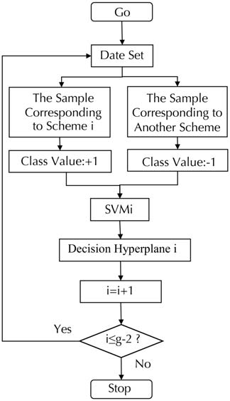
in Figure 5, the indirect method and combinatorial thinking are adopted in this study to build a binary tree
multi-level classifier. Let the scheme set of the sample be {scheme 0, scheme 1, scheme 2…, scheme g-1}.
The number of schemes is g. In Figure 6, the multi-level SVM classification model aims to differentiate all
schemes by combining multiple binary classifiers step by step.
l
D
o
w
N
o
UN
D
e
D
F
R
o
M
H
T
T
P
:
/
/
D
io
R
e
C
T
.
M
io
T
.
e
D
tu
D
N
/
io
T
/
l
UN
R
T
io
C
e
–
P
D
F
/
/
/
/
5
2
4
1
3
2
0
8
9
8
0
9
D
N
_
UN
_
0
0
2
0
8
P
D
T
.
/
io
F
B
sì
G
tu
e
S
T
T
o
N
0
7
S
e
P
e
M
B
e
R
2
0
2
3
Figura 5. The algorithm fl ow of multilevel classifi er.
Figura 6. The work fl ow of multilevel classifi er.
422
Data Intelligence
RS-SVM Machine Learning Approach Driven by Case Data for Selecting Urban Drainage
Network Restoration Scheme
4. EXPERIMENTS
We take the management practice of urban pipe network restoration project in Wuhu City, Anhui Province
as the background. Basing on sklearn.SVM and sklearn.metrics packages, we draw the conclusion by
comparing the RS-SVM machine learning method proposed in this paper with other algorithms (SVM
without attribute reduction, logistic algorithm without attribute reduction, logistic algorithm with attribute
reduction). The data set selected in this study contains 1500 samples, of which 1000 samples are randomly
selected as the training set and others as the test set. All experiments are conducted on a personal desktop
computer with 2 GHz Intel(R) Xeon (R) E5-2620 CPU, 8 GB RAM and Python 3.8.
4.1 Data Set
Referring to “Technical Specification for Inspection and Evaluation of Urban Drainage Pipes (CJ181-
2012) ", 68 conditional attributes {c1
P, c2
P, …, c68
P} are shown in Table 4.
Attribute
Code
Attribute
Code
Tavolo 4. Sixty-eight conditional attributes.
Pipe length
Buried depth
Pipe diameter
Material
Rupture I–IV
Interface material shedding I–IV
Branch pipe dark connection I–IV
Foreign body penetration I–IV
Leakage I–IV
Deposition I–IV
P
P
P
P
c1
P
c2
c3
c4
p–c8
p–c32
p–c36
p–c40
p–c44
p–c48
c5
c29
c33
c37
c41
c45
Transformation I–IV
Corrode I–IV
Wrong mouth I–IV
Ups and downs I–IV
Disconnect I–IV
Scaling I–IV
Obstacle I–IV
Residual wall and dam root I–IV
Root I–IV
Scum I–IV
P
P
P
P
P
P
c9
c13
c17
c21
c25
c49
c53
c57
c61
c65
p–c12
p–c16
p–c20
p–c24
p–c28
p–c52
p–c56
p–c60
p–c64
p–c68
P
P
P
P
P
P
P
P
P
l
D
o
w
N
o
UN
D
e
D
F
R
o
M
H
T
T
P
:
/
/
D
io
R
e
C
T
.
M
io
T
.
e
D
tu
D
N
/
io
T
/
l
UN
R
T
io
C
e
–
P
D
F
/
/
/
/
5
2
4
1
3
2
0
8
9
8
0
9
D
N
_
UN
_
0
0
2
0
8
P
D
.
T
/
io
The sample has four fixes. To facilitate differentiation, schemes are numbered in this study, and the
numbered values are taken as target attribute values, as shown in Table 5. According to Figure 6, three
classifiers should be built for the four schemes: SVM0, SVM1, and SVM2.
Tavolo 5. Value of each scheme target attribute.
Scheme
Not repair
Excavation and reconstruction
Ultraviolet light polymerization
Spot in situ curing
4.2 Data Standardization
Code
Scheme 0
Scheme 1
Scheme 2
Scheme 3
Value
0
1
2
3
To compress the data distribution, eliminate the impact of dimension, and improve the efficiency of
P)
attribute reduction and classification of SVM, we standardize the attribute values of pipeline material (c4
Data Intelligence
423
F
B
sì
G
tu
e
S
T
T
o
N
0
7
S
e
P
e
M
B
e
R
2
0
2
3
RS-SVM Machine Learning Approach Driven by Case Data for Selecting Urban Drainage
Network Restoration Scheme
according to Equation (1) and standardize those of other attributes according to Equation (2). Dopo
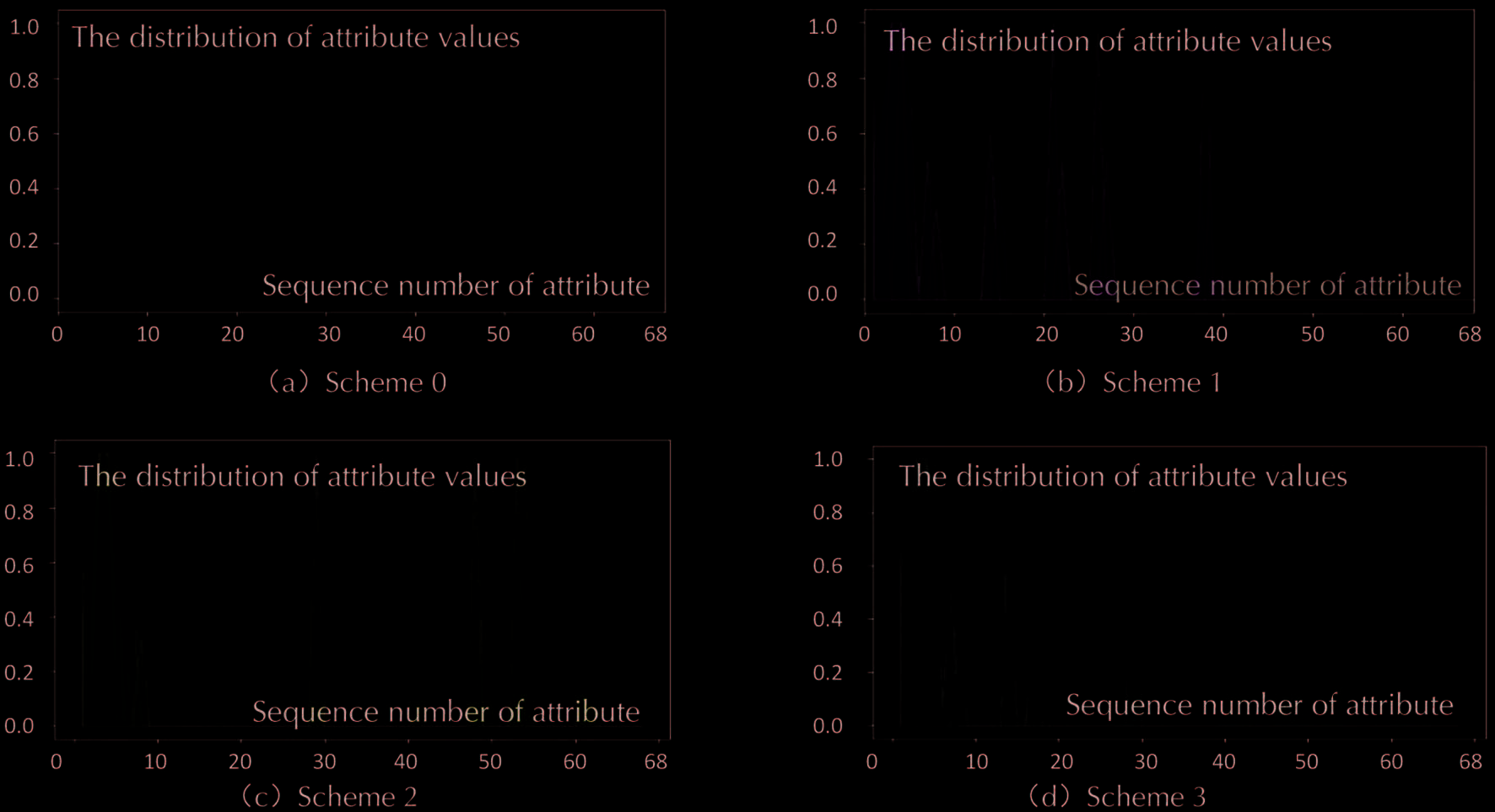
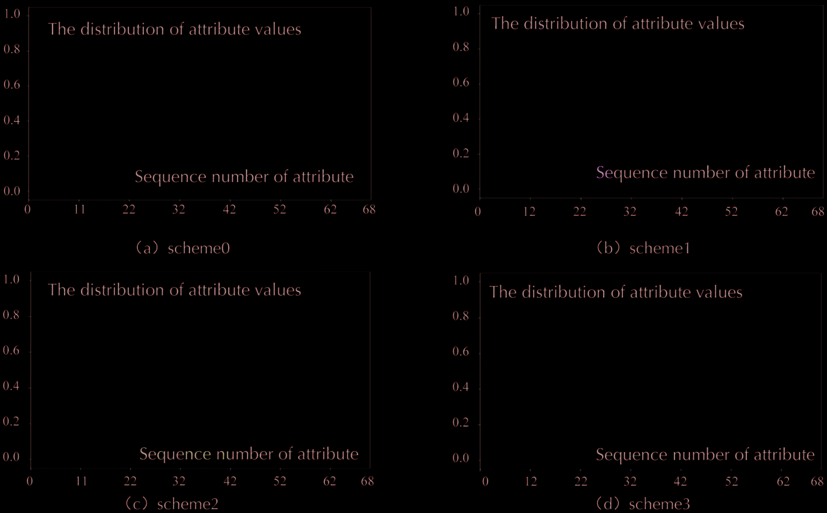
standardizing, the distribution of sample attribute values corresponding to the four repair schemes is shown
in Figure 7. In a repair scheme, the larger the sample size corresponding to the attribute value under an
attribute, the darker the color of the area. If the attribute value under an attribute corresponds to a smaller
sample size, the color of the area is lighter.
l
D
o
w
N
o
UN
D
e
D
F
R
o
M
H
T
T
P
:
/
/
D
io
R
e
C
T
.
M
io
T
.
e
D
tu
D
N
/
io
T
/
Figura 7. Distribution of attribute values of four restoration schemes.
l
UN
R
T
io
C
e
–
P
D
F
/
/
/
/
5
2
4
1
3
2
0
8
9
8
0
9
D
N
_
UN
_
0
0
2
0
8
P
D
/
T
.
io
4.3 Attributes Reduction
The pipeline defect type shown in Table 6 does not appear in all sample pipe segments of the pipeline
network repair project in Wuhu City, Anhui Province. Therefore, under the existing samples, the attributes
in Table 6 do not affect the selection of repair schemes and can be preliminarily reduced.
Attribute
Code
Attribute
Code
Tavolo 6. Type of defect not present in samples.
F
B
sì
G
tu
e
S
T
T
o
N
0
7
S
e
P
e
M
B
e
R
2
0
2
3
Deformation III
Metamorphosis IV
Etch IV
Misopening III
Foreign body is penetrated into IV
Leakage IV
Scaling III
Scaling IV
P
c11
c12
P
P
c16
c19
c40
c44
c51
c52
P
P
P
P
P
Mismouth IV
Disjunction IV
Interface material off IV
The branch pipe is secretly connected to IV
Residual wall and dam root I-IV
Root III
Root IV
Scum I-IV
P
P
P
P
c20
c28
c32
c36
p-c60
P
c63
c64
p-c68
P
P
P
c57
c65
424
Data Intelligence
RS-SVM Machine Learning Approach Driven by Case Data for Selecting Urban Drainage
Network Restoration Scheme
P, c7
P,c41
P,c35
P,c33
P,c27
P,c46
P,c37
P,c29
P,c39
P,c34
P,c38
P,c42
P,c26
P,c30
P, c3
P, c9
P,c48
P,c13
P,c49
P,c14
P,c50
P,c15
P,c53
P,c8
P,c47
P,c22
P,c61
P,c23
P,c18
P,c55
P,c4
P} , G2={core(),c4
P,D)>S(c10
P,
According to Equation (3)–(5), the core of the sample information system is obtained: core()={c2
P,c24
P,c21
P,c17
P,c25
P,c43
P, c6
c5
P,c45
P,c62
P,c56
P,c54
P}. According to Equation (6), the relatively necessary
P,c31
P, c10
P}. All reductions of the sample information system are
attributes are obtained: rna()={c1
P} , G3={core(),c10
P}. According to
P}, and G5={core(),c31
P}, G4={core(),c23
G1={core(),c1
P,D)>S(c23
P,D)>S(c1
P
Formula (7), S(c4
P,core()}. As IND(R)=IND(C) satisfies the indiscriminability
is first added to core() to form the set R={c4
P} is further reduced
P,c10
relation, R={c4
as a redundant attribute. Afterward, IL 42 attributes in R are sorted from smallest to largest according to
the subscript. The distribution of sample attribute values corresponding to the four repair schemes is shown
in Figure 8. The attribute numbers from 42 A 68 in Figure 8 is the redundant attribute set reduced, E
there is no peak value. By comparing Figures 7 E 8, we see that attribute reduction can remove redundancy
and compress and reduce the dimension of the distribution of data sets.
P, core()} is the relative minimalism of this example, E {c1
P,D); Perciò, the relatively necessary attribute c4
P,D)>S(c31
P,c31
P,c23
l
D
o
w
N
o
UN
D
e
D
F
R
o
M
H
T
T
P
:
/
/
D
io
R
e
C
T
.
M
io
T
.
e
D
tu
D
N
/
io
T
/
l
UN
R
T
io
C
e
–
P
D
F
/
/
/
/
5
2
4
1
3
2
0
8
9
8
0
9
D
N
_
UN
_
0
0
2
0
8
P
D
/
T
.
io
F
B
sì
G
tu
e
S
T
T
o
N
0
7
S
e
P
e
M
B
e
R
2
0
2
3
Figura 8. Sample attribute value distribution of the four restoration schemes after reduction.
4.4 Kernel Parameter Optimization
In recent years, many methods have been proposed by domestic and foreign experts and scholars to
evaluate the prediction effect of SVM, most of which are the Macro-Average-ROC [30]. The curves can be
used to qualitatively evaluate the prediction effect of different SVM classification models [31]. The area
Data Intelligence
425
RS-SVM Machine Learning Approach Driven by Case Data for Selecting Urban Drainage
Network Restoration Scheme
under the curve (Macro-Average-AUC) can quantitatively evaluate the prediction accuracy of different SVM
classification models. To facilitate the narration, we use MAR to represent Macro-Average-ROC and MAA
to represent Macro-Average-AUC.
Suppose the number of test samples is n and the number of categories is g. After the training is completed,
the probability of each test sample under each category is calculated and a matrix P with n rows and g
columns is obtained. Each line of P represents the probability value of a test sample under each category.
Accordingly, the labels of each test sample are converted to a binary like form. Each position is used to
mark whether it belongs to the corresponding category. Così, a label matrix L with n rows and g columns
can be obtained.
The basic idea of macro averaging is as follows: Under each category, you can get the probability that
n test samples are of that category (the columns in the matrix P). Therefore, according to each corresponding
column in the probability matrix P and label matrix L, false positive rate (FPR) and true positive rate (TPR)
under each threshold can be calculated, thus drawing a ROC curve. Così, a total of g ROC curves can be
plotted. FPR_all is obtained by merging, de-duplicating, and sorting all FPR of these ROC curves. The FPR
and TPR of the current class determine the ROC curve of the current class. The linear interpolation method
[32] is used to interpolate the horizontal coordinate that does not exist relative to FPR_all in FPR, and the
TPR’ after interpolation is obtained. TPR_mean is obtained by arithmetic averaging TPR’ after class g
interpolation. Finalmente, MAR curves are drawn according to FPR_all and TPR_mean. The equations of TPR_
mean and MAR are as follows:
TPR mean=
_
1
G
G
∑
i=
1
(
FPR_all ,FPR
interp
io
io
io
P
,T R )
MAA=
len(FPR_all)
∑
(TPR_mean +TPR_mean )(FPR_all
i+1
io
-FPR_all )/2
io
i+1
(20)
(21)
i=2
Am ong the four SVM kernel functions described in Section 3.3, we are uncertain which one is most
suitable for this data set. The parameter values of each kernel function are also uncertain. Così, the training
set containing 1000 samples is used to optimize the selection of the optimal kernel function and parameters,
as shown in Figure 1. Specifically, in the parameter definition domain, we draw an image of the MA A of
the model after attribute reduction as the parameter values changed (Figura 9) so as to determine the
optimal parameters of each kernel function after attribute reduction and the maximum MAA. A
compare and analyze the influence of attribute reduction on the SVM classification effect, we draw an
image of the model’s AUC changing with parameter values in the case of no attribute reduction (Figura 10).
We then determine the optimal parameter and maximum MAA of each kernel function without attribute
reduction.
426
Data Intelligence
l
D
o
w
N
o
UN
D
e
D
F
R
o
M
H
T
T
P
:
/
/
D
io
R
e
C
T
.
M
io
T
.
e
D
tu
D
N
/
io
T
/
l
UN
R
T
io
C
e
–
P
D
F
/
/
/
/
5
2
4
1
3
2
0
8
9
8
0
9
D
N
_
UN
_
0
0
2
0
8
P
D
T
.
/
io
F
B
sì
G
tu
e
S
T
T
o
N
0
7
S
e
P
e
M
B
e
R
2
0
2
3
RS-SVM Machine Learning Approach Driven by Case Data for Selecting Urban Drainage
Network Restoration Scheme
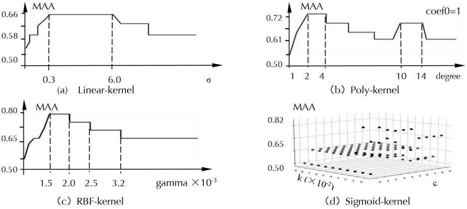
Figura 9. Parameter optimization results after attribute reduction.
l
D
o
w
N
o
UN
D
e
D
F
R
o
M
H
T
T
P
:
/
/
D
io
R
e
C
T
.
M
io
T
.
e
D
tu
D
N
/
io
T
/
l
UN
R
T
io
C
e
–
P
D
F
/
/
/
/
5
2
4
1
3
2
0
8
9
8
0
9
D
N
_
UN
_
0
0
2
0
8
P
D
T
.
/
io
F
B
sì
G
tu
e
S
T
T
o
N
0
7
S
e
P
e
M
B
e
R
2
0
2
3
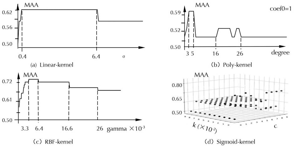
Figura 10. Parameter optimization results before attribute reduction.
(1) Linear kernel parameter optimization
The penalty coefficient σ is an important parameter of linear kernel function. The greater the σ is, IL
greater the penalty for misclassification. Hence, the accuracy of the training set is high, but the generalization
ability is weak. The smaller the σ value; the lower the penalty for misclassification, allowing fault tolerance,
and treating them as noise points; the stronger the generalization ability [33]. For linear kernel function,
before attribute reduction (Figura 10 (UN)), if 0<σ<0.4, the value of MAA increases with the increase of σ. If
Data Intelligence
427
RS-SVM Machine Learning Approach Driven by Case Data for Selecting Urban Drainage
Network Restoration Scheme
0.4≤σ≤6.4, MAA stabilizes around 0.62. If σ> 6.4, the data will be overfitted with the increase of σ, E
the value of MAA first decreases and then stabilizes around 0.56. After attribute reduction (Figura 9 (UN)), if
0<σ<0.3, the value of MAA increases with the increase of σ. If 0.3≤σ≤6.0, MAA stabilizes around 0.66. If
σ>6.0, the data are overfitted with the increase of σ, and the value of MAA first decreases and then stabilizes
around 0.58. Così, before attribute reduction, the optimal parameter interval of linear kernel is [0.4,6.4],
and then the value of MAA can reach 0.612. After attribute reduction, the optimal parameter interval of
linear kernel is [0.3,6.0], and then the value of MAA can reach 0.656.
(2) Poly kernel parameter optimization
High-order coefficients degree and coef0 are important parameters of the poly kernel function. IL
greater the degree, the higher the spatial dimension after mapping, the higher the complexity of calculating
the polynomial [34]. In particular, if degree=1 and coef0=0, the poly kernel is equivalent to the linear
kernel. In the case of coef0=1, we study the influence of degree on the classification accuracy of the poly
kernel function. Before attribute reduction (Figura 10 (B)), if 1≤degree≤3, the value of MAA increases with
the increase of degree. If 3≤degree≤5, the classification accuracy is stable at around 0.59. If 16≤degree≤26,
the MAA value fluctuates slightly between 0.51 E 0.53. With the increase of degree, the computational
complexity increases, and the value of MAA is stable around 0.51. After attribute reduction (Figura 9 (B)),
if 1≤degree≤2, the value of MAA increases with the increase of degree. If 2≤degree≤4, the value of MAA
is stable around 0.72. If 10≤degree≤14, MAA values show another peak, but this peak is slightly lower than
the first peak of 0.72. With the increase of degree, the computational complexity increases, and the value
of MAA is stable around 0.61. The optimal parameter interval of the poly kernel before attribute reduction
È [3,5], and then the value of MAA can reach 0.583. After attribute reduction, the optimal parameter
interval of the poly kernel is [2,4], and then the value of MAA can reach 0.716.
(3) RBF kernel parameter optimization
l
D
o
w
N
o
UN
D
e
D
F
R
o
M
H
T
T
P
:
/
/
D
io
R
e
C
T
.
M
io
T
.
e
D
tu
D
N
/
io
T
/
l
UN
R
T
io
C
e
–
P
D
F
/
/
/
/
5
2
4
1
3
2
0
8
9
8
0
9
D
N
_
UN
_
0
0
2
0
8
P
D
T
.
/
io
Gamma, an important parameter of the RBF kernel function, controls the penalty threshold range and
mainly defines the influence of a single sample on the entire classification hyperplane. If gamma is small,
a single sample has little influence on the whole classification hyperplane, so selecting it as a support vector
is hard. Conversely, a single sample has a greater impact on the whole classification hyperplane and is
more likely to be selected as a support vector, or the whole model will have more support vectors [33]. In
this study, the optimal gamma value is searched within [103,+∞), and the search ends when the value of
MAA becomes stable with the increase of gamma. Before attribute reduction (Figura 10 (C)), if
0
