RECHERCHE
Functional connectivity of fMRI using differential
covariance predicts structural connectivity
and behavioral reaction times
Yusi Chen1,2
, Qasim Bukhari3, Tiger W. Lin1,4, and Terrence J. Sejnowski1,2,5
1Computational Neurobiology Laboratory, Salk Institute for Biological Sciences, La Jolla, Californie, Etats-Unis
2Division of Biological Studies, University of California San Diego, La Jolla, Californie, Etats-Unis
3McGovern Institute for Brain Research, Massachusetts Institute of Technology, Cambridge, MA, Etats-Unis
4Neurosciences Graduate Program, University of California San Diego, La Jolla, Californie, Etats-Unis
5Institute for Neural Computation, University of California San Diego, La Jolla, Californie, Etats-Unis
un accès ouvert
journal
Mots clés: Functional connectivity, Resting-state fMRI, Differential covariance, Human
Connectome Project
ABSTRAIT
Recordings from resting-state functional magnetic resonance imaging (rs-fMRI) reflect the
influence of pathways between brain areas. A wide range of methods have been proposed to
measure this functional connectivity (FC), but the lack of “ground truth” has made it difficult
to systematically validate them. Most measures of FC produce connectivity estimates that
are symmetrical between brain areas. Differential covariance (dCov) is an algorithm for
analyzing FC with directed graph edges. When we applied dCov to rs-fMRI recordings
from the human connectome project (HCP) and anesthetized mice, dCov-FC accurately
identified strong cortical connections from diffusion magnetic resonance imaging (dMRI) dans
individual humans and viral tract tracing in mice. En outre, those HCP subjects whose
dCov-FCs were more integrated, as assessed by a graph-theoretic measure, tended to have
shorter reaction times in several behavioral tests. Ainsi, dCov-FC was able to identify
anatomically verified connectivity that yielded measures of brain integration significantly
correlated with behavior.
RÉSUMÉ DE L'AUTEUR
Our ability to sense, think, feel and react is reflected in the activation patterns of distinct brain
régions. These patterns can be observed noninvasively by functional magnetic resonance
imaging (IRMf). Statistical dependencies between the activities in brain regions have been
widely used to measure functional connectivity (FC). Cependant, due to common inputs from
other brain areas, two correlated brain regions may not have direct neural fibers connecting
eux, which makes correlated activity difficult to interpret. A new method for measuring
FC called differential covariance (dCov) was applied to fMRI recordings from anesthetized
mice and resting human subjects. The analysis closely matched known neuronal fiber
relations. En outre, dCov-FC from individual humans predicted reaction times for
several types of psychological tests.
Citation: Chen, Y., Bukhari, Q., Lin,
T. W., & Sejnowski, T. J.. (2022).
Functional connectivity of fMRI using
differential covariance predicts
structural connectivity and behavioral
reaction times. Neurosciences en réseau,
6(2), 614–633. https://est ce que je.org/10.1162
/netn_a_00239
EST CE QUE JE:
https://doi.org/10.1162/netn_a_00239
Informations complémentaires:
https://doi.org/10.1162/netn_a_00239
Reçu: 12 Juillet 2021
Accepté: 10 Février 2022
Intérêts concurrents: Les auteurs ont
a déclaré qu'aucun intérêt concurrent
exister.
Auteur correspondant:
Terrence J. Sejnowski
terry@salk.edu
Éditeur de manipulation:
Randy McIntosh
droits d'auteur: © 2022
Massachusetts Institute of Technology
Publié sous Creative Commons
Attribution 4.0 International
(CC PAR 4.0) Licence
La presse du MIT
je
D
o
w
n
o
un
d
e
d
F
r
o
m
h
t
t
p
:
/
/
d
je
r
e
c
t
.
m
je
t
.
t
/
/
e
d
toi
n
e
n
un
r
t
je
c
e
–
p
d
je
F
/
/
/
/
/
6
2
6
1
4
2
0
2
8
1
3
0
n
e
n
_
un
_
0
0
2
3
9
p
d
.
t
F
b
oui
g
toi
e
s
t
t
o
n
0
7
S
e
p
e
m
b
e
r
2
0
2
3
dCov-FC predicts structural connectivity and behavioral measurements
Functional connectivity (FC):
Statistical relationship between
recorded neural entities; could be
inferred using different methods.
INTRODUCTION
Functional connectivity (FC) is a measure of how brain regions interact with each other during
resting-state functional magnetic resonance imaging recordings (rs-fMRI). The definition of FC
has shifted from association to causation, which was previously referred to as effective
connectivité (Reid et al., 2019). To be consistent with the prevailing definition, we refer to
all estimated connectivity patterns, whether causal or not, as FC. Methods for computing
FC have been tested on synthetic data, but testing on fMRI recordings is problematic without
ground truth. New approaches are needed using other sources of evidence.
Promising new methods have been developed for extracting FC from fMRI data, y compris
Granger causality (Granger, 1969) and dynamic causal modeling (DCM) (Friston, Harrison, &
Penny, 2003). Granger causality uses a linear autoregressive model to quantify connectivity in
terms of temporal dependencies. DCM uses a generative model to infer the causal latent states
underlying the observations. Regression dynamic causal modeling (rDCM) was recently
developed assuming that the dynamics are linear. These methods have advanced our under-
standing of FC but they are computationally demanding and have a large number of param-
eters (K. Stephan, Iglesias, Heinzle, & Diaconescu, 2015). Here we explore a new FC method
that is scalable to very large datasets while maintaining good performance.
je
D
o
w
n
o
un
d
e
d
F
r
o
m
h
t
t
p
:
/
/
d
je
r
e
c
t
.
m
je
t
.
/
t
/
e
d
toi
n
e
n
un
r
t
je
c
e
–
p
d
je
F
/
/
/
/
/
6
2
6
1
4
2
0
2
8
1
3
0
n
e
n
_
un
_
0
0
2
3
9
p
d
.
t
F
b
oui
g
toi
e
s
t
t
o
n
0
7
S
e
p
e
m
b
e
r
2
0
2
3
The covariance matrix is the most commonly used method to calculate FC and is compu-
tationally efficient (Smith et al., 2011); cependant, two correlated nodes may not have a direct
physical connection because of covariance propagation (Stevenson, Rebesco, Miller, &
Conduite, 2008). Partial covariance reduces indirect correlations but not interactions due to
unobserved common inputs. These spurious connections produced by covariance-based
methods make it harder to interpret the links between FC and the underlying physiological
states. En outre, covariance is a symmetric matrix, which is not consistent with functional
dependencies that are not symmetric.
Differential covariance (dCov), which is the focus of this study, reduces false positive connec-
tions and recovers the ground truth connectivity from data generated by simulated models (Lin
et coll., 2020; Lin, Le, Krishnan, Bazhenov, & Sejnowski, 2017).1 Compared with other statistical
méthodes, dCov seeks to estimate connectivity from a dynamical system perspective. It makes use
of the derivative signal, in addition to the original signal, to capture the dynamical interactions
between neural measurements and is, in general, not a symmetric matrix. When recorded neural
responses are viewed as a dynamical system governed by a set of ordinary differential equations,
the derivative provides information about the moving trend of the state variables. By evaluating
the relationship between the derivative signal and the original signal, we can link the current
state to future states, and thus extract the directed connectivity pattern (Chiffre 1). The goal of this
article is to apply dCov to rs-fMRI recordings to evaluate its performance compared with other
FC methods in predicting structural connectivity and behavioral data.
Some studies have focused on validating FC on several known projections or subnetworks,
such as the default mode network (DMN) (Parc, Friston, Pae, Parc, & Razi, 2018), but leave
open the validity of the larger FC matrix. Since direct activity dependencies between two
brain regions depend on fiber projections connecting them, it is reasonable to expect the
FC to be closely related to the underlying structural connectivity (SC) (Vincent et al., 2007),
with the strength depending on brain dynamics. We used SC obtained through either viral
1Note that the acronym dCov-FC refers to functional connectivity revealed by differential covariance. Ce
should not be confused with the distance covariance based upon pairwise distances between random vari-
ables (https://en.wikipedia.org/wiki/ Distance_correlation).
615
Differential covariance (dCov):
The novel method of estimating
directed functional connectivity,
including three matrices described in
“Theoretical Background.”
Structural connectivity (SC):
Structural connection strength that
can be experimentally measured.
Spécifiquement, it refers to tracing
strength in the mouse dataset and
fiber density in the HCP dataset.
Neurosciences en réseau
dCov-FC predicts structural connectivity and behavioral measurements
Chiffre 1. Differential covariance estimates the influence of source activity on changes in the
sink activity. The output from the source area is driven by VB and the input to the sink area is given
dt , which is related to the input currents, IA, by the Hodgkin–Huxley equation. The covariance
by dVA
between these two signals is a measure of the directed flow of information from the sources to
the sinks.
tracing in mice or diffusion magnetic resonance imaging (dMRI) in humans as surrogates for
“ground truth.”
Although the existence of anatomical connections, either direct or indirect, is a necessary con-
dition for the dynamic coupling of neuronal activities between two brain regions, neural activity
dependencies are more dynamic and variable than the underlying anatomical linkages. Honey
et autres. (2009) systematically examined the relationship between Pearson correlation–based FC
and diffusion tensor imaging (DTI) based SC at high spatial resolution. They pointed to the redun-
dancy and unreliability of structurally unconnected functional connections. Since then, major
efforts have been made to predict FC from SC (Abdelnour, Dayan, Devinsky, Thesen, & Raj,
2018; Abdelnour, Voss, & Raj, 2014; Grandjean, Zerbi, Balsters, Wenderoth, & Rudin, 2017;
Messé, Rudrauf, Giron, & Marrelec, 2015). But these approaches typically accounted for less than
half of the known structural connections (Grandjean et al., 2017). A complete match from the
entire weighted FC matrix to the weighted SC matrix is difficult to achieve owing to limitations
of both FC estimation and DTI. To obtain a better match between FC and SC, we chose to focus
on examining the subset of significant functional connections. This also had the advantage of
increasing the tolerance of FC estimation to various noise sources in fMRI recordings (Liu, 2016).
Another challenge is to gain insights from the estimated FCs into how behavior is generated
in brains. Methods from network science, especially those rooted in graph theory, have been
useful for analyzing the dynamics of how information is communicated in brains (Avena-
Koenigsberger, Misic, & Sporns, 2018). Several core concepts describing the segregation
and integration of information (Sporns, 2013) have provided insights into cognitive control
mechanisms (Cohen & D'Esposito, 2016; Marek, Hwang, Foran, Hallquist, & Luna, 2015;
Santarnecchi, Galli, Polizzotto, Rossi, & Rossi, 2014) and brain disorders (Huang, Wu, Lin,
Pang, & Chen, 2019). This suggests that the topological properties of FCs evaluated by different
methods could provide new insights into brain function.
To extract the most reliable signals, we binarized FC and SC and systematically compared
FC defined by dCov with commonly used FC estimation methods, quantifying performance by
their correspondence with anatomically strong connections. The resulting FC matrices were
also topologically analyzed and compared with behavioral measurements to link them with
brain states that give rise to behavior.
Neurosciences en réseau
616
je
D
o
w
n
o
un
d
e
d
F
r
o
m
h
t
t
p
:
/
/
d
je
r
e
c
t
.
m
je
t
.
/
/
t
e
d
toi
n
e
n
un
r
t
je
c
e
–
p
d
je
F
/
/
/
/
/
6
2
6
1
4
2
0
2
8
1
3
0
n
e
n
_
un
_
0
0
2
3
9
p
d
t
.
F
b
oui
g
toi
e
s
t
t
o
n
0
7
S
e
p
e
m
b
e
r
2
0
2
3
dCov-FC predicts structural connectivity and behavioral measurements
COMPUTATIONAL BACKGROUND
The differential covariance method makes use of the derivative signal. In most models of
neural dynamics, the derivative of a neuron’s membrane potential is related to its incoming
synaptic and intrinsic currents (c'est à dire., sinks), and its own membrane potential is related to its
output (c'est à dire., sources) (Chiffre 1). Differential covariance uncovers the relationship between
sinks and sources. In this paper, we calculated three dCov matrices: differential covariance
matrice, Δc (Supporting Information Figure S1, Équation 1); partial differential covariance
matrice, Δp (Supporting Information Figure S1, Équation 2); and sparse-latent regularized partial
differential covariance matrix, Δs (Supporting Information Figure S1, Équation 3). We briefly
introduce here these three measures and further discuss them along with other measures in the
Methods section below.
The differential covariance Δc is defined in Equation 1, where zi is the time trace of node i
in a network, dzi is the numerical derivative of zi (the superscript bar denotes the sample mean
of a time trace), and cov denotes the estimation of sample covariance between two time traces.
(cid:1)
Δcij ¼ cov dzi; zj
(cid:3)
¼ 1
T − 1
XT
(cid:1)
t¼1
dzi tð Þ − (cid:1)
dz i
(cid:3)
(cid:1)
(cid:3)
zj tð Þ − (cid:1)zj
(1)
je
D
o
w
n
o
un
d
e
d
F
r
o
m
h
t
t
p
:
/
/
d
je
r
e
c
t
.
m
je
t
.
Node:
Neural entity being recorded. Ici, it
refers to a group of voxels belong to
the same independent component.
t
/
/
e
d
toi
n
e
n
un
r
t
je
c
e
–
p
d
je
F
/
/
/
/
/
6
2
6
1
4
2
0
2
8
1
3
0
n
e
n
_
un
_
0
0
2
3
9
p
d
t
.
F
b
oui
g
toi
e
s
t
t
o
n
0
7
S
e
p
e
m
b
e
r
2
0
2
3
The partial differential covariance Δp can be calculated in Equation 2, where K is the set of
nodes other than i and j; Cov is the covariance matrix; CovjK 2 ℝ1×(N−2), CovKK 2 ℝ(N−2)×(N−2);
and ΔciK 2 ℝ1×(N−2).
Δpij ¼ Δcij − CovjK Cov−1
KK
ΔcT
iK
(2)
The partial differential covariance controls the effects of confounding variables by calculat-
ing the relationship based on residual time traces, paralleling the derivation of the partial
covariance matrix (Cox & Wermuth, 2014). In most cases, the residual time traces were
obtained by solving a multiple linear regression problem with confounding variables included
as independent variables.
The third matrix, Δs, minimizes the effects of latent inputs from outside the recorded regions,
which are not uncommon in fMRI recordings. We adopted a sparse latent regularization method
to separate Δp into a sparse matrix Δs and a low-rank matrix L. Under reasonable assumptions,
the sparse matrix represents direct coupling between observed nodes and the low-rank matrix
represents the residual effects from unobserved nodes (Yatsenko et al., 2015). We obtained Δs by
solving a constrained optimization problem using an augmented Lagrangian multiplier (Candès,
Li, Ma, & Wright, 2011). The objective function is the weighted sum between L1-norm of the
vectorized sparse matrix and the trace of the low-rank matrix. The penalty ratio α controls
the sparsity of Δs. We fixed α to 1ffiffiffi
p because this choice provides an almost exact solution to
N
the sparse matrix separation problem (Theorem 1.1 in Candès et al., 2011):
Constrain : Δp ¼ Δs þ L
Δs ¼ arg min
Δs
(cid:1)
Δsk
k
1
(cid:3)
þ α (cid:2) tr Lð Þ
(3)
These three differential covariance matrices reduce three types of common false positive
relations (Figure 2B). To be more specific, Δc deals with errors due to confounder effects
(Figure 2B1). In the calculation of Δp, both confounder (Figure 2B1) and chain effects
(Figure 2B2) are taken into account. The sparser Δs further reduces the effect of latent con-
founders (Figure 2B3).
Neurosciences en réseau
617
dCov-FC predicts structural connectivity and behavioral measurements
je
D
o
w
n
o
un
d
e
d
F
r
o
m
h
t
t
p
:
/
/
d
je
r
e
c
t
.
m
je
t
.
/
t
/
e
d
toi
n
e
n
un
r
t
je
c
e
–
p
d
je
F
/
/
/
/
/
6
2
6
1
4
2
0
2
8
1
3
0
n
e
n
_
un
_
0
0
2
3
9
p
d
.
t
F
b
oui
g
toi
e
s
t
t
o
n
0
7
S
e
p
e
m
b
e
r
2
0
2
3
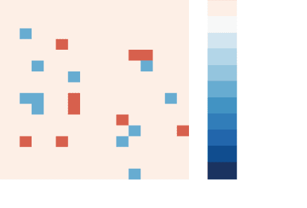
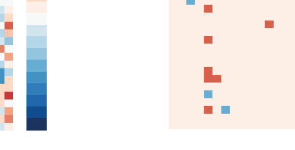
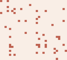
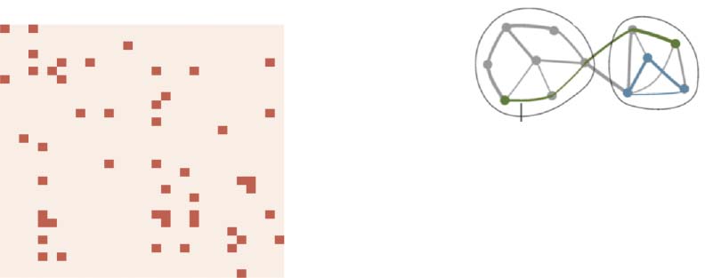
Chiffre 2. Workflow and features of differential covariance-based methods. (UN) Workflow. Two-way arrows mean that we compared the
boxed quantities. (B) Differential covariance-based methods have been shown to effectively reduce the three types of errors in network model-
ing shown in B1, B2, and B3 (Lin et al., 2017). Black solid lines denote actual physical connections and red dashed lines denote false positive
correlational relationship. B1: confounder effects due to common input; B2: chain effects due to propagation; B3: latent confounders due to
unobserved common inputs. (C) The partial differential covariance matrix, Δp, on the left and its binarized matrix on the right (binarization
threshold = 0.01) of one mouse subject. Partial differential covariance matrices are directed, nonsymmetric, and sparser than the correspond-
ing covariance matrices (Supporting Information Figure S1).
Neurosciences en réseau
618
dCov-FC predicts structural connectivity and behavioral measurements
RÉSULTATS
Functional Connectivity Estimated by Differential Covariance
We followed standard procedures for preprocessing fMRI recordings (Smith et al., 2013).
Voxel-wise time traces were decomposed into component-wise time traces and MRI maps
je
D
o
w
n
o
un
d
e
d
F
r
o
m
h
t
t
p
:
/
/
d
je
r
e
c
t
.
m
je
t
.
/
/
t
e
d
toi
n
e
n
un
r
t
je
c
e
–
p
d
je
F
/
/
/
/
/
6
2
6
1
4
2
0
2
8
1
3
0
n
e
n
_
un
_
0
0
2
3
9
p
d
t
.
F
b
oui
g
toi
e
s
t
t
o
n
0
7
S
e
p
e
m
b
e
r
2
0
2
3
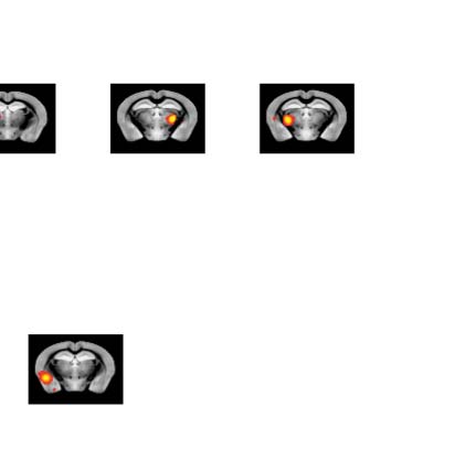
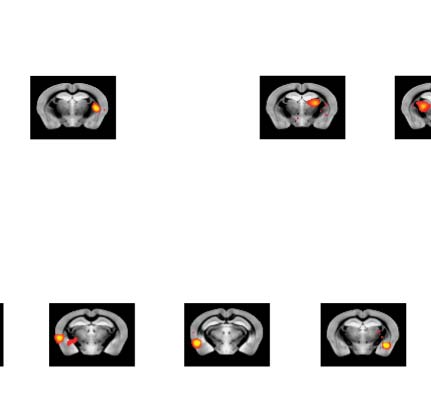
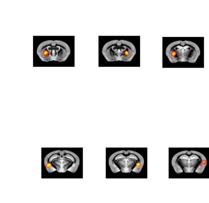
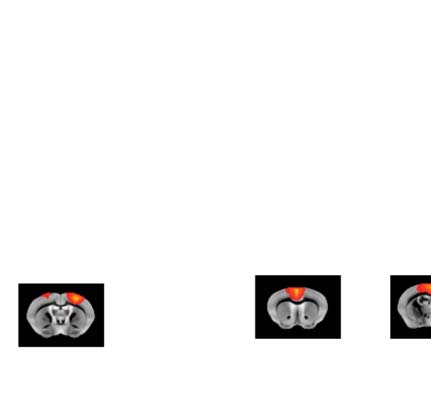
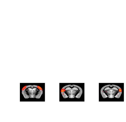
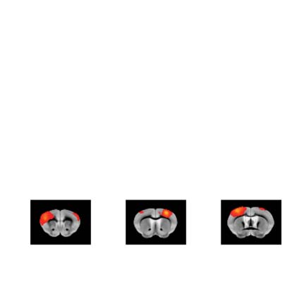
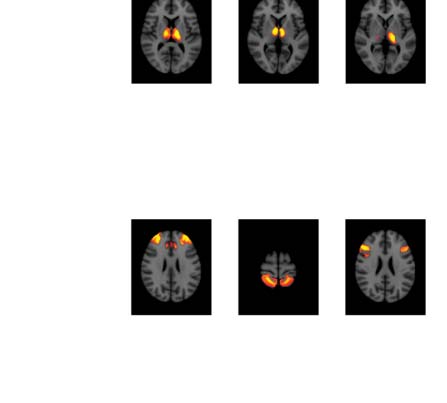
Chiffre 3. Significant Δp-FC connections shared across subjects and associated MRI spatial maps
from the mouse rs-fMRI dataset. (UN) For Δp-FC estimated from the mouse dataset, relations
which are significant (binarization threshold = 0.01) in more than 2 sujets (out of 12) were plot
in the circular plot. (B) MRI spatial maps of the independent components were grouped into sub-
réseaux. The registered anatomical locations were shown underneath. Note that there could be
more than one component (Par exemple, component 17 et 19) corresponding to the same ana-
tomical region due to the unsupervised nature of group ICA. S1, primary somatosensory cortex; S2,
secondary somatosensory cortex; M1, primary motor cortex; dACC, dorsal anterior cingulate cortex;
Cg, cingulate cortex; RSG, retrosplenial cortex; Amy, amygdalar; Ect, entorhinal cortex; PRh, peri-
rhinal; CPu, caudoputamen; Ins, insular; pir, piriform; GP, Globus Pallidus; dTh, dorsal thalamus;
vTh, ventral thalamus. Refer to Supporting Information Table S3 for detailed annotations.
Neurosciences en réseau
619
dCov-FC predicts structural connectivity and behavioral measurements
of each component through group independent component analysis (ICA) and dual regression
(Figure 2A) (Methods). After manually removing artifactual components, the remaining
components (30 for mouse and 60 for HCP) were registered with corresponding anatomical
locations in a brain atlas (MRI maps are shown in Figure 3 and Figure 4; annotations are
shown in Supporting Information Table S2 and Table S3). This preprocessing yielded an
je
D
o
w
n
o
un
d
e
d
F
r
o
m
h
t
t
p
:
/
/
d
je
r
e
c
t
.
m
je
t
.
/
t
/
e
d
toi
n
e
n
un
r
t
je
c
e
–
p
d
je
F
/
/
/
/
/
6
2
6
1
4
2
0
2
8
1
3
0
n
e
n
_
un
_
0
0
2
3
9
p
d
t
.
F
b
oui
g
toi
e
s
t
t
o
n
0
7
S
e
p
e
m
b
e
r
2
0
2
3
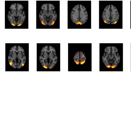
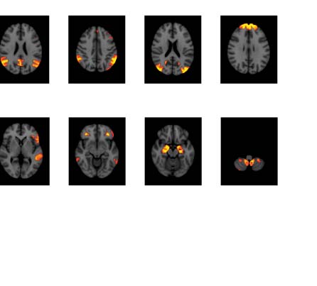
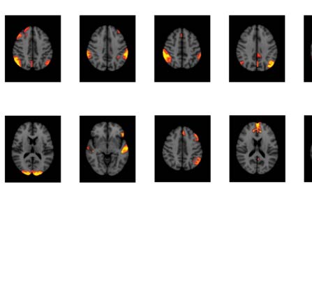
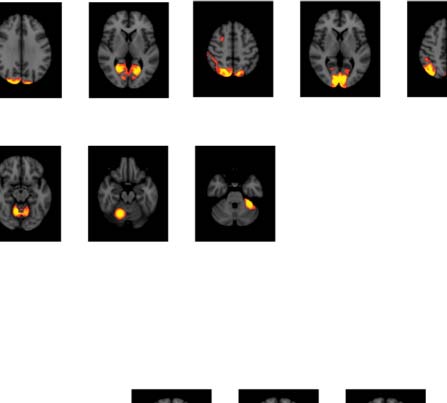
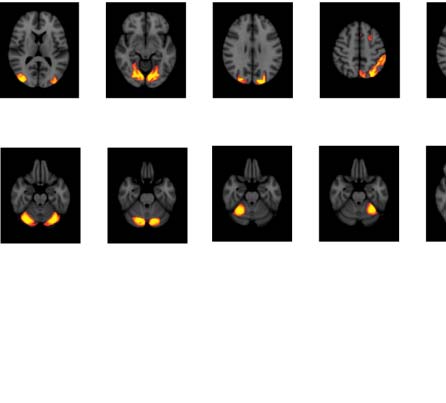
Chiffre 4. Significant Δp-FC connections shared across subjects and associated MRI spatial maps from the HCP rs-fMRI dataset. (UN) For Δp-FC
estimated from the HCP dataset, connections that are significant (binarization threshold = 0.01) in more than 30 sujets (out of 1,003) étaient
plot in the circular plot. (B) MRI spatial maps of the independent components were grouped into subnetworks. The number marks the index of
the independent components. The indices are from 1 à 100, but only 60 of them were shown here because the remaining components were
treated as imaging artifacts. Refer to Supporting Information Table S2 for more detailed annotations.
Neurosciences en réseau
620
dCov-FC predicts structural connectivity and behavioral measurements
N × T (number of components × number of time points) matrix representing time-varying hae-
modynamic signals for various anatomical locations. We then applied a recently developed
backward reconstruction method to reconstruct neural signals (z) from haemodynamic signals
(example time traces shown in Supporting Information Figure S4). Backward reconstruction
based on the forward Balloon model (Friston, Mechelli, Tourneur, & Prix, 2000) has been shown
to work well together with dCov applied to synthetic datasets (Lin et al., 2020).
Functional connectivity (FC) matrices (N × N ) were estimated from the reconstructed neural
signals, z, using popular FC estimation methods, together with the three dCov matrices men-
tioned above. The benchmarked estimators (Methods) include the sample covariance matrix
(Cov), the precision matrix (Pcov), L1-/L2-regularized precision matrix (L1-/L2-reg), and con-
ditional Granger causality (cGranger). En général, dCov matrices give rise to FC matrices that
are not symmetric, and are antisymmetric for Δc, which could, in practice, potentially predict
the direction of information flow (Supporting Information Figure S1).
To reduce the susceptibility of FC matrices to noise, we determined the significance level of
connections by using a bootstrap procedure (except for cGranger whose significance level was
calculated through χ2 distribution). The null hypothesis is that activities of all the nodes in the
network are generated independently and, as a consequence, there are no statistical relation-
ships between any node pair within the null dataset. An autoregressive (AR) bootstrap proce-
dure (Efron & Tibshirani, 1986; Nalci, Rao, & Liu, 2019) was used to generate the null time
traces to preserve the power spectral density of haemodynamic signals, and then null FCs were
estimated from the null time traces. For each empirical connection, the probability that its
value belongs to the null distribution, its p value, was calculated assuming the distribution
was Gaussian. Thresholds of significance were applied to binarize the FC matrix so that we
could focus on a set of significant connections. Because dCov-based methods intrinsically
reduce false positive connections, they yielded fewer significant connections compared to
covariance-based methods (Supporting Information Figure S1).
We applied the above workflow to extract FCs from fMRI recordings in anesthetized mice
and resting-state recordings from the HCP dataset. The mouse dataset included 12 sujets,
and the HCP dataset included 1,003 young adult subjects. Figures 3B and 4B show the MRI
spatial maps of each component. Due to the individual variability of connectivity patterns, le
circular plots in Figures 3A and 4A only showed the subset of significant connections shared
across subjects. Components were allocated into networks according to their corresponding
anatomical locations. The first inspection of shared connections showed promising correspon-
dence between Δp-FC and the anatomical wiring of different brain regions. Par exemple, dans
Chiffre 3, Δp-FC picked up important connections within the mouse lateral cortical network,
which is located in the densely interconnected Module 2 (M2) subsystem reported by
Swanson et al. (2018) (M2 is shown in Figure 3 of the reference paper). In Figure 4, the visual
network is densely interconnected across multiple subjects revealed by Δp-FC. Donc, nous
next quantified the similarity between dCov-FC and SC at individual level and population level
in human and mouse subjects, respectivement.
Differential Covariance FC More Closely Matches the Underlying Structural Connections
We developed a pipeline to systematically quantify the similarity between FC and SC. We first
constructed an N × N structural connectivity, “ground truth” matrix, with nodes corresponding
to the anatomical regions that matched the independent components obtained from resting-
state recordings (Supporting Information Figure S2 and Figure S3, Methods). We used the exist-
ing SC database for the connectivity profiles between different anatomical regions.
Neurosciences en réseau
621
je
D
o
w
n
o
un
d
e
d
F
r
o
m
h
t
t
p
:
/
/
d
je
r
e
c
t
.
m
je
t
.
t
/
/
e
d
toi
n
e
n
un
r
t
je
c
e
–
p
d
je
F
/
/
/
/
/
6
2
6
1
4
2
0
2
8
1
3
0
n
e
n
_
un
_
0
0
2
3
9
p
d
.
t
F
b
oui
g
toi
e
s
t
t
o
n
0
7
S
e
p
e
m
b
e
r
2
0
2
3
dCov-FC predicts structural connectivity and behavioral measurements
Spécifiquement, we used population level viral tracing data (Swanson et al., 2018) for mouse SC
and individual level dMRI data (Rosen & Halgren, 2021) for human SC (Methods). The mouse
“ground truth” matrix (Supporting Information Figure S2) is not symmetric while the human
“ground truth” matrices (Supporting Information Figure S3) are symmetric and sparse with sub-
stantial amount of individual variability. In both cases, higher values indicate higher structural
connectivity strength. We then calculated the average structural connectivity strength (ASCS)
of the set of significant connections picked through AR bootstrapping under multiple binari-
zation thresholds. The decreasing binarization threshold provides a stricter criterion for con-
nection selection and pictures an asymptotic description of the evaluated quantity. A higher
ASCS value implies that a specific FC more closely matched the underlying SC.
We calculated ASCS values for FC defined by the covariance matrix (cov), partial covari-
ance matrix (Pcov), regularized partial covariance matrix (L1/L2-reg), conditional Granger
causality (cGranger), differential covariance matrix (Δc), partial differential covariance matrix
(Δp), and sparse differential covariance matrix (Δs). Figure 5B and 5D show ASCS values of
significant connections, using multiple binarization thresholds, pooled from all subjects in
mouse and HCP dataset, respectivement.
In both mouse (Figure 5B) and human datasets
(Figure 5D), Δp and Δs had significantly (p < 0.05, rank-sum test) higher ASCS values than
those based on benchmark methods. Figure 5A and 5C showing structural connectivity
strength (SCS) distributions from one individual subject revealed a reduced number of low-
SCS connections in both Δp and Δs. This is a consequence of the method’s ability to reduce
false positive connections, as previously shown using synthetic data in simulation studies (Lin
et al., 2020). In general, dCov-FC produced sparse estimation, which contributed to its higher
ACSC values. Even at the same sparsity level, Δs still showed significantly higher ASCS com-
pared to all other methods (Supporting Information Figure S7). This means that in addition to
sparsity, there are other favorable statistical properties that enable dCov to capture important
anatomical connections.
Differential Covariance FC Measures the Integration of Brain Activity
Next, we wanted to know whether dCov-based FC matrices, which are aligned with the under-
lying SC, could also provide insights into the interpretation of behavioral measurements. The
HCP dataset (Methods) consists of not only high-quality macroscopic-level imaging data, but
also hundreds of behavioral measurements, including detailed psychological test results from
1,003 young adult subjects (Van Essen et al., 2013). The large sample size and the full assess-
ment of subjects’ psychological states render the HCP dataset an invaluable source for
investigating the organizing principles linking human brain networks and behavioral readouts.
We calculated several topological properties of the FC matrices (Rubinov & Sporns, 2010).
Because of the inherent interdependencies and transitivity of bivariate methods, the covari-
ance matrix is not suitable for calculating network properties (Avena-Koenigsberger et al.,
2018). So FC derived from the partial correlation matrix (Pcov-FC) was used for control.
Pcov-FC and Δs-FC exhibited similar network properties such as network degree distribution
(Supporting Information Figure S5A), clustering behavior, transitivity, and modularity proper-
ties (Supporting Information Figure S5C) across subjects. In addition, both Pcov-FC and Δs-FC
showed similar network degree distribution to that of population level diffusion tensor imaging
network reported in Hagmann et al. (2008) (Supporting Information Figure S5B). Surprisingly,
the network efficiency of Δs-FC is strongly anticorrelated (r = 0.71) with that of Pcov-FC
(Figure 6A). Network efficiency, calculated as the average of the inverse path length of shortest
signaling routes between two nodes (Methods), measures the network’s integration level. Since
622
Average structural connectivity
strength (ASCS):
Average of SCS. This was used as a
measure of similarity between FC
and SC.
Structural connectivity
strength (SCS):
The set of structural connectivity
strength of the statistically significant
functional connections.
Network efficiency:
Average of the inverse path length of
the shortest path between two nodes.
A measure of network integration.
Network Neuroscience
l
D
o
w
n
o
a
d
e
d
f
r
o
m
h
t
t
p
:
/
/
d
i
r
e
c
t
.
m
i
t
.
t
/
/
e
d
u
n
e
n
a
r
t
i
c
e
-
p
d
l
f
/
/
/
/
/
6
2
6
1
4
2
0
2
8
1
3
0
n
e
n
_
a
_
0
0
2
3
9
p
d
t
.
f
b
y
g
u
e
s
t
t
o
n
0
7
S
e
p
e
m
b
e
r
2
0
2
3
dCov-FC predicts structural connectivity and behavioral measurements
l
D
o
w
n
o
a
d
e
d
f
r
o
m
h
t
t
p
:
/
/
d
i
r
e
c
t
.
m
i
t
.
/
/
t
e
d
u
n
e
n
a
r
t
i
c
e
-
p
d
l
f
/
/
/
/
/
6
2
6
1
4
2
0
2
8
1
3
0
n
e
n
_
a
_
0
0
2
3
9
p
d
.
t
Figure 5. Differential covariance (dCov)-FC preferentially identified connections with high SCS in both mouse and HCP dataset. (A and C)
The SCS distribution of the significant (binarization threshold: p < 0.01) connections identified by different methods from recordings of one
mouse subject (A) or one human subject in the HCP dataset (C). Δp and Δs identified connections with higher SCS. (B and D) Under different
binarization thresholds, ASCS of the significant connections pooled from all subjects in the mouse dataset (B) and the HCP dataset (D). Under
all binarization thresholds, Δp and Δs have better performance than the baseline methods in picking up structurally connected regions. FC,
functional connectivity; cov, covariance; Pcov, partial covariance; L1/L2-reg, L1/L2-norm regularized partial covariance; cGranger, condi-
tional Granger causality; Δc, differential covariance; Δp, partial differential covariance; Δs, partial differential covariance with sparse latent
regularization.
f
b
y
g
u
e
s
t
t
o
n
0
7
S
e
p
e
m
b
e
r
2
0
2
3
Δs-FC reduces false positive connections/paths in the network, it selects for the important and
reliable routes and decreases redundant routes. As a consequence, network efficiency of
Δs-FC could potentially be a better description of the integration level.
To investigate this hypothesis, we compared this measure of network integration with each
subject’s fluid intelligence quantified by their reaction time to the test. This behavioral mea-
surement has been previously shown to be most related to FC (Smith et al., 2015). One expects
that a higher level of network integration would lead to shorter reaction times, and indeed
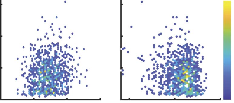
Δs-FC–based global efficiency is inversely correlated (r = −0.14) to reaction time (Figure 6B).
As a control, we sorted the correlations between Δs-FC–based global efficiency and all behav-
ioral measurements after controlling common influencing factors like age and brain size. Five
Network Neuroscience
623
dCov-FC predicts structural connectivity and behavioral measurements
l
D
o
w
n
o
a
d
e
d
f
r
o
m
h
t
t
p
:
/
/
d
i
r
e
c
t
.
m
i
t
.
t
/
/
e
d
u
n
e
n
a
r
t
i
c
e
-
p
d
l
f
/
/
/
/
/
6
2
6
1
4
2
0
2
8
1
3
0
n
e
n
_
a
_
0
0
2
3
9
p
d
t
.
f
b
y
g
u
e
s
t
t
o
n
0
7
S
e
p
e
m
b
e
r
2
0
2
3
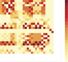
Figure 6. Differential covariance based FC matrices could be a more reasonable measurement of the integration level of the brain. (A) In the
HCP dataset, global efficiency of Δs-FC and Pcov-FC are strongly anti-correlated (r = 0.71). (B) Global efficiency of Pcov-FC is positively
correlated (left, r = 0.15, p = 1.2e−6) to the reaction time of fluid intelligence task while the global efficiency of Δs-FC is negatively correlated
(right, r = −0.14, p = 1.4e−5) to it. In most cases, we would expect a negative correlation because the more highly integrated the network,
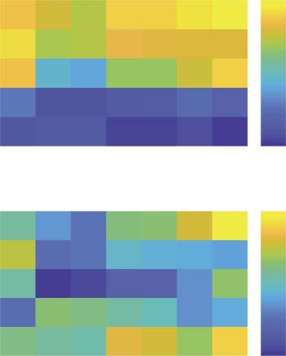
the shorter the response time. Color scale codes for the density of the samples. (C) The table lists the behavioral measurements that are
most significantly correlated ( p < 0.001) to the global efficiency of Δs-FC, after controlling for confounding factors. Most of the significant
behavioral measurements are related to reaction time in different tasks (shown in bold). Heat maps below show their correlation values and
p values.
out of seven significant (p < 0.005) behavioral measurements are reaction time in various
psychological tests (Figure 6C), which further confirmed the significance of Δs-FC as a mea-
sure of the integration of brain activity.
DISCUSSION
In this article, we applied three variants of dCov to estimate FC from rs-fMRI recordings. Com-
pared to the covariance matrix, differential covariance identified a subset of connections with
high structural connectivity strength, largely owing to dCov’s ability to reduce three types of
false positive connections. These results were confirmed in both human and mouse record-
ings. In addition, by ruling out redundant signaling routes, the sparse-latent regularized partial
differential covariance matrix (Δs-FC) provided the closest link to behavioral measurements
Network Neuroscience
624
dCov-FC predicts structural connectivity and behavioral measurements
and functional network integration based on the inverse of shortest path length, a measure of
global efficiency.
The estimates of directed connectivity afforded by dCov-FC are formally related to the esti-
mates of effective connectivity from dynamic causal modeling, under linear assumptions,
because dCov-FC rests upon the same generative model used in rDCM (Frässle et al., 2017).
However, interactions are estimated using variational Bayesian inference in dynamic causal
modeling (Friston et al., 2003), whereas dCov-FC expresses the interaction pattern in terms
of the covariance between the derivative signal and the original signal. Without the need to
go through the model fitting process, dCov is a much faster and more straightforward algorithm.
The current versions of dCov assume that the underlying system is linear and that the con-
nectivity pattern is closely related to the adjacency matrix in graph theory or transition matrix
in dynamical system analysis. Although the computational processes in brains are by no
means linear, the averaging of activity in large neural populations, as in the case of fMRI
recordings, is approximately linear (Stephan et al., 2008). The current linear dCov estimator
could be extended to nonlinear estimators, taking into account the threshold firing properties
of individual neurons, to better extract connectivity at the single neuron level (Chen, Rosen, &
Sejnowski, 2021).
The calculation of sparse-latent regularized partial differential covariance matrix (Δs) used
a method for sparse-latent regularization that was initially proposed by Yatsenko et al. (2015)
and Candès et al. (2011). This sparse-latent regularization assumes a sparse structure of the
intrinsic connections and a low-rank component representing common fluctuations and com-
mon latent inputs. This assumption may or may not be fulfilled in fMRI recordings, and there is
no straightforward way to test this assumption. Nonetheless, the addition of sparse latent reg-
ularization did not influence the qualitative conclusions (compare Δp and Δs in Figure 5 and
Figure 6C).
There are potential biases that may be introduced by using structural connectivity as the
ground truth. First, the connection strengths revealed by the tractography-based measurements
used in the HCP dataset decay exponentially with tract length (Rosen & Halgren, 2021), thus
likely underestimating long-distance connections (Jones, Knösche, & Turner, 2013); Second,
we used individual-level dMRI matrices for the HCP dataset to account to individual variabil-
ity. These matrices are sparser compared to the population average. Finally, dMRI fails to
reveal the direction of structural connections and the population level SC matrix constructed
from mouse viral tracing is almost symmetric. These concerns limited the accuracy of compar-
isons between the directed connections inferred by dCov methods and the dMRI dataset.
Recent efforts have been made toward a dynamic description of directed connectivity, such
as dynamic effective connectivity (Zarghami & Friston, 2020), and dCov is another step toward
this direction. First, the derivative signal reflects a dynamical description of the system (Chen
et al., 2021) and is also used in regression dynamic causal modeling (rDCM) (Frässle et al.,
2017). In comparison, dCov is more intuitive and faster than rDCM. Second, a sliding-window
approach has been used to compute time-dependent covariance matrices (Hutchison et al.,
2013), aiming to capture context-dependent fluctuations in the functional connectivity.
However, due to the stationarity assumption required by sample covariance estimation, fluc-
tuations in the covariance matrix may imply a violation of stationarity rather than a measure of
switching between brain states. Nor does a static covariance matrix imply the absence of
switching (Liegeois, Laumann, Snyder, Zhou, & Yeo, 2017). In contrast, dCov does not require
stationarity so that, in principle, applying a sliding-window analysis together with dCov could
provide a more accurate description of the changes in regional coupling.
Network Neuroscience
625
l
D
o
w
n
o
a
d
e
d
f
r
o
m
h
t
t
p
:
/
/
d
i
r
e
c
t
.
m
i
t
.
/
/
t
e
d
u
n
e
n
a
r
t
i
c
e
-
p
d
l
f
/
/
/
/
/
6
2
6
1
4
2
0
2
8
1
3
0
n
e
n
_
a
_
0
0
2
3
9
p
d
.
t
f
b
y
g
u
e
s
t
t
o
n
0
7
S
e
p
e
m
b
e
r
2
0
2
3
dCov-FC predicts structural connectivity and behavioral measurements
In conclusion, in addition to validating dCov’s performance on fMRI recordings, we have
also extended previous studies linking FC to connectivity and behavior. The analytic tech-
niques for studying links to anatomy and behavior introduced here can be applied to other
methods for determining FC and other datasets, which could provide stronger confidence in
their interpretation.
METHODS
Data Acquisition and Preprocessing
We used two rs-fMRI datasets, including an anesthetized mouse dataset first reported in
Bukhari et al. (2018) and the extensively processed young adult rs-fMRI S1200 dataset from
Human Connectome Project (https://www.humanconnectome.org).
For the mouse dataset, experiment and imaging protocols were defined in the original
publication. For all 12 animals, each subject received approximately 1.2% Isoflurane (Abbott,
Cham, Switzerland) with a tolerance of 0.1% in a 20% oxygen/80% air mixture. The data was
collected in two sessions, where the animals remained inside the scanner during the whole
time. The total time series acquired during the two sessions were of 680-s length. Subjects
were scanned using a Bruker Biospec 94/30 small animal MR system (Bruker BioSpin MRI,
Ettlingen, Germany) operating at 400 MHz (9.4 T). A gradient-echo echo-planar imaging
(GE-EPI) sequence has been used for rs-fMRI data acquisition with field of view = 16 ×
7 mm2, matrix dimensions = 80 × 35, TR = 1 second, TE = 12 ms, flip angle = 60 degree.
Each subject had 680 imaging frames collected.
All the preprocessing was performed using tools from FMRIB’s Software Library (FSL version
5). FSL’s recommended pre-processing pipeline was used. Motion correction, removal of non-
brain structures, high-pass temporal filtering with sigma = 75.0 s, prewhitening, and global
spatial smoothing using a 0.2-mm Gaussian kernel was applied to increase signal-to-noise
ratio as part of the preprocessing. After the preprocessing, the functional scans were aligned
to the high-resolution anatomical AMBMC template (https://www.imaging.org.au/AMBMC
/AMBMC) using linear affine and nonlinear diffeomorphic transformation registration as imple-
mented in ANTs (ANTs. v 1.9; https://picsl.upenn.edu/ANTS/). We used FSL’s MELODIC for
probabilistic independent component analysis. The multisession temporal ICA concatenated
approach, as recommended for rs-fMRI data analysis, allowed to input all subjects from all the
groups in a temporally concatenated fashion for the ICA analysis. ConcatICA yielded different
activations and artifact components without the need of specifying any explicit time series
model. A total of 100 independent components (IC maps) were extracted, and the mixture
model approach was applied on these estimated maps to perform inference analysis. An alter-
native hypothesis test based on fitting a Gaussian/gamma mixture model to the distribution of
voxel intensities within spatial maps 53 and 54 was used to threshold the IC maps. A threshold
of 0.5 ( p < 0.5) was selected for the alternative hypothesis in order to assign equal ‘cost’ to
false positives and false negatives. Out of the 100 independent components (IC maps), only 30
were selected, while the components that overlapped with vascular structures and ventricles
were excluded from further analysis. Similarly, regions at the brain surface, which are prone to
be affected by the motion artifacts due to, for example, breathing, were excluded.
For the HCP dataset, we used the extensively processed “HCP1200 Parcellation +
Timeseries + Netmats (1003 Subjects)” dataset available through the website. Detailed prepro-
cessing and study design could be easily accessed through the website. In this release, 1,003
healthy adult human subjects (ages 22–37 years, 534 females) were scanned on a 3-T Siemens
connectome-Skyra scanner (customized to achieve 100 mT m−1 gradient strength). Each
Network Neuroscience
626
l
D
o
w
n
o
a
d
e
d
f
r
o
m
h
t
t
p
:
/
/
d
i
r
e
c
t
.
m
i
t
.
t
/
/
e
d
u
n
e
n
a
r
t
i
c
e
-
p
d
l
f
/
/
/
/
/
6
2
6
1
4
2
0
2
8
1
3
0
n
e
n
_
a
_
0
0
2
3
9
p
d
.
t
f
b
y
g
u
e
s
t
t
o
n
0
7
S
e
p
e
m
b
e
r
2
0
2
3
dCov-FC predicts structural connectivity and behavioral measurements
subject underwent 4 × 15 minutes recording sessions with temporal resolution of 0.73 second
and spatial resolution of 2 mm isotropic. Subject-specific measures including behavioral,
demographic, and psychometric measures are available from the HCP data dictionary.
For imaging data processing, each 15-minute run of each subject’s rs-fMRI data was pre-
processed according to Smith et al. (2013); it was minimally preprocessed (Glasser et al.,
2013), and had artefacts removed using ICA + FIX (Griffanti et al., 2014; Salimi-Khorshidi
et al., 2014). Intersubject registration of cerebral cortex was carried out using areal feature–
based alignment and the multimodal surface matching algorithm (MSMAll) (Glasser et al.,
2016; Robinson et al., 2014). Each dataset was temporally demeaned and had variance nor-
malization and then fed into the MIGP algorithm, whose output is the top 4,500 weighted
spatial eigenvectors from a group-averaged PCA (a very close approximation to concatenating
all subjects’ time series and then applying PCA) (Smith, Hyvärinen, Varoquaux, Miller, &
Beckmann, 2014). The MIGP output was fed into group-ICA using FSL’s MELODIC tool,
applying at several different dimensionalities (D = 25, 50, 100, 200, 300). In our analysis,
we used a 100-dimensional decomposition because the number of parcellation nodes used
in multiple studies was typically around 100 (Dadi et al., 2019).
Component Specific Time Series
For a given “parcellation” (group-ICA map), the set of ICA spatial maps was mapped onto each
subject’s rs-fMRI time series data to derive one representative time series per ICA component
per subject. This process was fulfilled by the standard “dual-regression stage-1” approach, in
which the full set of ICA maps was used as spatial regressors against the full data (Filippini
et al., 2009). This results in an N × T (number of components × number of time points) matrix
for each subject. Thus, we consider each ICA component as a network “node.” These time
series can then be used to reveal statistical relationship in a network, as will be described
in section Estimation of Functional Connectivity.
Reconstruction of Neural Activity
Before estimating the functional connectivity, we adopted two methods to reconstruct neural
signals z from haemodynamic time series y, which was obtained from the dual regression pro-
cess described above.
Backward reconstruction. Backward reconstruction was developed based on a biophysical
model which transforms neural activities to BOLD signals via a set of differential equations
(Stephan, Weiskopf, Drysdale, Robinson, & Friston, 2007). One important step in this model
links blood flow to BOLD signal through a Balloon model assumption. Therefore, in this
article, we will refer to this entire biophysical process as the forward Balloon model. The
backward reconstruction process linearizes the equations and derives a surrogate neural signal
z as a linear combination of haemodynamic signals y and its ith order derivatives y(i ) (Equation 4)
(Khalidov, Fadili, Lazeyras, Van De Ville, & Unser, 2011). Note that according to the linearized
Balloon model, the reconstructed surrogate signal z is a linear combination of real neural signal
V and its first order derivative V_,
z ¼ q1V_þ q0V
¼ p4y 4ð Þ þ p3y 3ð Þ þ p2y 2ð Þ þ p1 _y þ p0y
(4)
where the coefficients pi and qi are functions of biophysical parameters: τ, (cid:2), α, κ, γ, ϑ0, ρ, η, and
V0 (Equation 5). Some parameter values vary with respect to magnetic field strength (B). Please
refer to Supporting Information Table S1 for annotations of these biophysical parameters and
Network Neuroscience
627
l
D
o
w
n
o
a
d
e
d
f
r
o
m
h
t
t
p
:
/
/
d
i
r
e
c
t
.
m
i
t
.
/
t
/
e
d
u
n
e
n
a
r
t
i
c
e
-
p
d
l
f
/
/
/
/
/
6
2
6
1
4
2
0
2
8
1
3
0
n
e
n
_
a
_
0
0
2
3
9
p
d
t
.
f
b
y
g
u
e
s
t
t
o
n
0
7
S
e
p
e
m
b
e
r
2
0
2
3
dCov-FC predicts structural connectivity and behavioral measurements
the specific values used in this paper. Most values were taken from Stephan et al. (2007) unless
cited. We also demonstrated that the backward reconstruction process is robust to a wide
range of parameter values in simulation tests (data not shown).
Þτη − k3 − k2
ð
ð
Þη
Þ τ − 1 þ α
ατ
ÞηV0
ð
− k3 − k2
τ
Þη
V0
ð
q1 ¼ − k1 þ k2
ð
q0 ¼ − k1 þ k2
k1 ¼ 4:3ϑ0ρTE
k2 ¼ (cid:2)r0ρTE
k3 ¼ 1 − (cid:2)
p4 ¼ τ
p3 ¼ 1 þ 1
α
(cid:5)
p2 ¼ 1
þ τγ þ 1 þ 1
τα
α
(cid:5)
p1 ¼ 1 þ 1
α
γ
p0 ¼
τα
κ
τα
þ τκ
γ þ
(cid:6)
(cid:6)
κ
(5)
Blind deconvolution. Blind deconvolution is an alternative method to remove effects of hemo-
dynamic response from rs-fMRI recordings (Wu et al., 2013). The basic idea is to consider the
fluctuations of rs-fMRI as ‘spontaneous event-related,’ individuate point processes correspond-
ing to signal fluctuations with a given signature, extract a region-specific hemodynamic
response function and use it for deconvolution. Details and implementation could be found
in the original article (Wu et al., 2013).
Estimation of Functional Connectivity
Functional connectivity is represented by a N × N matrix, which describes the statistical rela-
tionship of N node time series. To quantify this relationship, we adopted commonly used
covariance-based algorithms, Granger causality, and three novel differential covariance based
algorithms.
Covariance based methods. Denote the entire N node time series as a N × T matrix with each
row vector as zi, then entry (i, j ) of the covariance matrix Cov 2 ℝN×N could be calculated
as follows:
(cid:1)
Covij ¼ cov zi; zj
(cid:3)
¼ 1
T − 1
XT
zik − z(cid:1)i
ð
(cid:1)
Þ zjk − z(cid:1)j
(cid:3)
k¼1
(6)
where the superscript bar denotes the sample mean of a time trace and cov denotes the
estimation of sample covariance between two time traces.
The partial covariance matrix Pcov 2 ℝN×N, also called the precision matrix, aims to esti-
mate direct connections more accurately than the full covariance matrix. Pcov is the inverse of
the covariance matrix:
Pcov ∝ Cov−1
(7)
Regularized partial covariance. Regularization methods can be implemented during the regres-
sion step of calculating partial covariance matrix when the connectivity matrix is sparse. We
calculated L1- and L2-regularized partial covariance matrices through the FSL toolbox
(Jenkinson, Beckmann, Behrens, Woolrich, & Smith, 2012) using default values for the penal-
izing parameter: λ = 10 for L1-regularization and ρ = 0.1 for L2-regularization. For both
Network Neuroscience
628
l
D
o
w
n
o
a
d
e
d
f
r
o
m
h
t
t
p
:
/
/
d
i
r
e
c
t
.
m
i
t
.
/
t
/
e
d
u
n
e
n
a
r
t
i
c
e
-
p
d
l
f
/
/
/
/
/
6
2
6
1
4
2
0
2
8
1
3
0
n
e
n
_
a
_
0
0
2
3
9
p
d
t
.
f
b
y
g
u
e
s
t
t
o
n
0
7
S
e
p
e
m
b
e
r
2
0
2
3
dCov-FC predicts structural connectivity and behavioral measurements
methods, we varied these regularization parameters, and there was no significant difference in
performance over a wide range of values (Supporting Information Figure S8).
Granger causality. Granger causality (Granger, 1969) is a statistical interpretation of causality
based on predictability: A is said to “Granger cause” B if the predictability of B declines when
A is removed from the predictors. The test of predictability increase or decline typically uses a
multivariate vector autoregressive model. We implemented conditional Granger causality
(cGranger) through the MVGC MATLAB toolbox (Barnett & Seth, 2014). In this approach,
the fundamental assumption is that the time series data is a realization of a stationary vector
autoregressive process. The vector autoregressive model order was chosen based on Akaike
information criterion and the coefficients of the full/reduced regression model was computed
through ordinary least square solution to the regression. For significance test of Granger cau-
sality, the G-causality estimator scaled by sample size has an asymptotic χ2 distribution under
the null hypothesis of zero causality. The reported p values were before multiple test
correction.
Differential covariance based methods. Differential covariance–based methods are a set of algo-
rithms developed to extract direct connections in a network, especially under the influence of
common inputs and latent inputs. The calculation of dCov-based FC was detailed in section of
main text on Computational Background. In our previous work (Lin et al., 2017, 2020), the
advantages of differential covariance–based methods over covariance-based methods have
been fully demonstrated both analytically and numerically. Readers can refer to our previous
work for more details.
Significance Testing of FC
To assess the statistical significance of the relationship between hemodynamic signals, we
used an autoregressive (AR) bootstrap procedure (Efron & Tibshirani, 1986; Nalci et al.,
2019) to preserve the power spectrum density of hemodynamic signals. For a specific connec-
tion, denoted as element (i, j ) of the above FC matrices, our null hypothesis was that BOLD
signal zi and zj were generated independently regardless of other nodes’ time traces. To gen-
erate null time series, we fit separate AR processes of model order q to node-specific time
traces. The model order q was determined according to the Bayesian information criterion.
A higher order model was rejected if it could not decrease Bayesian information criterion
by more than 2. Using the estimated AR coefficients of empirical time series, we generated
1,000 surrogate null time series and then computed the associated functional connectivity cor-
responding to the null hypothesis. For each connection, we assumed a Gaussian distribution of
the null connectivity values. P value was calculated as the probability of the empirical FC
value that appeared under the null Gaussian distribution. In this paper, we didn’t correct for
multiple comparison and instead adopted different significance levels as binarization
thresholds.
Structural Connectivity Matrix
SC matrix was constructed as an N × N matrix with each node corresponding to the anatom-
ical regions represented by one IC map. To construct the structural connectivity matrix for
mouse subjects, we first manually identified the anatomical regions shown on each IC map
and then pulled out their connectivity profiles from the existing SC database. If one IC map
corresponds to multiple anatomical locations in the database, following the method in
Hagmann et al. (2008), we calculated the average connectivity strength of these locations
as the connectivity strength of this IC map. The adopted SC database quantified axonal
Network Neuroscience
629
l
D
o
w
n
o
a
d
e
d
f
r
o
m
h
t
t
p
:
/
/
d
i
r
e
c
t
.
m
i
t
.
/
t
/
e
d
u
n
e
n
a
r
t
i
c
e
-
p
d
l
f
/
/
/
/
/
6
2
6
1
4
2
0
2
8
1
3
0
n
e
n
_
a
_
0
0
2
3
9
p
d
.
t
f
b
y
g
u
e
s
t
t
o
n
0
7
S
e
p
e
m
b
e
r
2
0
2
3
dCov-FC predicts structural connectivity and behavioral measurements
connections within rat cerebral cortex and nuclei (Swanson et al., 2018). Connection strength
was quantified from 1 = lowest to 7 = highest. The database was built upon a systematic
review of neuro-anatomical literature reporting tracing results. The diagonal of mouse SC
matrix was set to 7 because intraregional connections are intensive and there is limited liter-
ature reporting intraregional tracing.
For the SC of human subjects, we used the individual level SC matrices constructed in our
previous work (Chen et al., 2021; refer to method 4.3 in the reference). In short, we used prob-
abilistic diffusion tractography to evaluate the dMRI measurements (Rosen & Halgren, 2021).
The mapping between ICs and dMRI measurements was performed at voxel level. Only 46
HCP components were used in the FC-SC analysis since dMRI measurements were restricted to
cortical voxels. Readers could refer to Supporting Information Table S3 (mouse) and Table S2
(HCP) for the identified anatomical regions of each IC map.
FC and SC Comparison
The comparison of FC and SC was quantified through structual connectivity strength (SCS) and
its average (ASCS). SCS refers to the set of structural connectivity strength of the significant
functional connections. In practice, we binarized difference FC matrices through their signif-
icance level, creating a boolean mask of the SC matrix. The the selected SC values were
integrated into the SCS set until such procedure was repeated in all involved subjects. The
distribution of the SCS set was plotted in Figure 5A and C. The average value of this SCS
set (ASCS) was used as a measure of similarity of SC and FC. ASCS of different methods were
plotted in Figure 5B and D.
Network Topological Analysis
For the HCP dataset, the estimated FC matrices were binarized (threshold = 0.05) and then
assessed using topological network measurements so that we could characterize the FC network
by using several neuro-biologically meaningful and easily computable measurements (Rubinov &
Sporns, 2010). These measurements include node degree (ki), global efficiency (E ), clustering
Table 1. Mathematical definition of network topological measure for (un)directed graphs
Measure
(Out)-degree (ki)
In-degree (k in
i
)
Shortest path length (dij)
Number of triangles (ti)
Global efficiency (E )
Local efficiency (Eloc)
Clustering coefficient (C )
Transitivity (T )
Modularity (Q)
Network Neuroscience
Definition for Undirected Graph
(cid:3)j2N aij
Definition for Directed Graph
(cid:3)j2N aij
/
(cid:3) auv, auv 2 gi↔j
(cid:3)j,h aijaihajh
1
2
1
2
P
(cid:3)j2N aji
(cid:3) auv, auv 2 gi→j
(cid:3)j,h (aij + aji)(aih + ahi)(ajh + ahj)
P
aij aihd −1
Þ
i;j2N;j≠h
ð
ki ki −1
ð
jh Ni
1
N
(cid:3)i2N
1
N
(cid:3)i2N Ei = 1
N
(cid:3)i2N
j2N;j≠i
N−1
d −1
ij
P
Þ
1
2N
(cid:3)i2N
Þ aihþahi
ð
ð
aij þaji
i;j2N;j≠h
ð
Þ k out
ð
þk in
k out
þk in
i
i
i
i
(cid:1)
Þ d −1
ð
jh Ni
P
Þ−2
−1
Þþd −1
ð
hj Ni
aij aji
j
(cid:3)
Þ
1
N
(cid:3)i2N
P
2ti
ð
ki ki −1
Þ
P
2ti
i2N
Þ
ki ki −1
ð
i2N
1
N
(cid:3)i2N
ð
k out
i
þk in
i
Þ k out
ð
P
i
ti
þkin
i
−1
P
Þ−2
aij aji
j
ð
k out
i
þk in
i
ð
Þ k out
i
ti
i2N
þkin
−1
i
P
Þ−2
aij aji
j
(cid:3)u2M [euu − ((cid:3)v2M euv)]2
630
l
D
o
w
n
o
a
d
e
d
f
r
o
m
h
t
t
p
:
/
/
d
i
r
e
c
t
.
m
i
t
.
/
t
/
e
d
u
n
e
n
a
r
t
i
c
e
-
p
d
l
f
/
/
/
/
/
6
2
6
1
4
2
0
2
8
1
3
0
n
e
n
_
a
_
0
0
2
3
9
p
d
t
.
f
b
y
g
u
e
s
t
t
o
n
0
7
S
e
p
e
m
b
e
r
2
0
2
3
dCov-FC predicts structural connectivity and behavioral measurements
coefficient (C), transitivity (T ), local efficiency (Eloc), and modularity (Q). All the measurements
were computed using brain connectome toolbox (https://sites.google.com/site/bctnet/). For a
binarized network with N nodes, these quantities were defined in Table 1 for undirected graphs
(Pcov-FC) and directed graphs (Δs-FC): where aij 2 {0, 1} refers to the existence of network edges,
dij refers to shortest path length between two nodes (dij = ∞ if not connected), and ti is the
number of local triangles around node i. In the calculation of modularity (Q), the network
was fully subdivided into a set of nonoverlapping modules M, and euv is the proportion of
all links that connect nodes in module u with nodes in module v. It can be verified that these
measures for undirected graphs are special cases of those for directed graphs in which aij = aji.
To compare the topological properties of different FC matrices, we calculated the correlation
E, C, T, Eloc, and Q between Pcov-FC and Δs-FC across all subjects (Supporting Information
Figure S5C). For each individual subject, the node (out)-degree distribution of the Pcov-FC, Δs-FC
and and diffusion tensor imaging (Hagmann et al., 2008) networks were fitted by a Gaussian
distribution, a power law distribution (small value truncated), and an exponential distribution
using maximum likelihood estimation (Supporting Information Figure S5A). For Δs-FC (directed
graph), the distributions for the node in-degree and out-degree were very similar and Gaussian
distributed (Supporting Information Figure S6). The distributions of k in
i + ki for directed graphs
and 2ki for undirected graphs are shown in Supporting Information Figure S5A.
To evaluate the relationship between global network efficiency (E ) and behavioral measure-
ments (BM), we first combined all the BMs documented in the public dataset and restricted
dataset (both available by download from the HCP website), resulting in a matrix of size 1003 ×
408 = 409,224 (number of subjects × number of BMs). Then in reference to Smith et al.
(2015), we identified five confounding BMs, including age, weight, height, blood pressure-
systolic, blood pressure-diastolic, and total brain volume. All these confounding BMs were
regressed out of the network efficiency measurements E so that we only focused on the resid-
ual efficiency values. We further excluded BMs with more than 200 missing data points. The
Pearson correlation between residual efficiency and BMs are calculated, and BMs are sorted
according to the significance of their correlation between Δs-FC (Figure 6C).
SUPPORTING INFORMATION
Supporting information for this article is available at https://doi.org/10.1162/netn_a_00239.
ACKNOWLEDGMENTS
We thank Dr. Thomas Liu for helpful discussions and for suggesting to look for behavioral cor-
relates of dCov. The authors would like to thank Burke Rosen, Javier How, Robert Kim, Ben
Tsuda, and other CNL members for helpful discussion and feedback. The authors also thank
Jorge Aldana for assistance with computing resources.
REFERENCES
Abdelnour, F., Dayan, M., Devinsky, O., Thesen, T., & Raj, A.
(2018). Functional brain connectivity is predictable from ana-
tomic network’s Laplacian eigen-structure. NeuroImage, 172,
728–739. https://doi.org/10.1016/j.neuroimage.2018.02.016,
PubMed: 29454104
Abdelnour, F., Voss, H. U., & Raj, A. (2014). Network diffusion
accurately models the relationship between structural and func-
tional brain connectivity networks. NeuroImage, 90, 335–347.
https://doi.org/10.1016/j.neuroimage.2013.12.039, PubMed:
24384152
Avena-Koenigsberger, A., Misic, B., & Sporns, O. (2018). Commu-
nication dynamics in complex brain networks. Nature Reviews
Neuroscience, 19(1), 17–33. https://doi.org/10.1038/nrn.2017
.149, PubMed: 29238085
Barnett, L., & Seth, A. K. (2014). The MVGC multivariate granger
causality toolbox: A new approach to Granger-causal inference.
Network Neuroscience
631
l
D
o
w
n
o
a
d
e
d
f
r
o
m
h
t
t
p
:
/
/
d
i
r
e
c
t
.
m
i
t
.
/
/
t
e
d
u
n
e
n
a
r
t
i
c
e
-
p
d
l
f
/
/
/
/
/
6
2
6
1
4
2
0
2
8
1
3
0
n
e
n
_
a
_
0
0
2
3
9
p
d
t
.
f
b
y
g
u
e
s
t
t
o
n
0
7
S
e
p
e
m
b
e
r
2
0
2
3
dCov-FC predicts structural connectivity and behavioral measurements
Journal of Neuroscience Methods, 223, 50–68. https://doi.org/10
.1016/j.jneumeth.2013.10.018, PubMed: 24200508
Bukhari, Q., Schroeter, A., & Rudin, M. (2018). Increasing isoflur-
ane dose reduces homotopic correlation and functional segrega-
tion of brain networks in mice as revealed by resting-state fMRI.
Scientific Reports, 8(1), 10591. https://doi.org/10.1038/s41598
-018-28766-3, PubMed: 30002419
Candè s, E. J., Li, X., Ma, Y., & Wright, J. (2011). Robust principal
component analysis? Journal of the ACM ( JACM), 58(3), 1–37.
https://doi.org/10.1145/1970392.1970395
Chen, Y., Rosen, B. Q., & Sejnowski, T. J. (2021). Dynamical differ-
ential covariance recovers directional network structure in multi-
scale neural systems. bioRxiv. https://doi.org/10.1101/2021.06
.18.448901
Cohen, J. R., & D’Esposito, M. (2016). The segregation and integra-
tion of distinct brain networks and their relationship to cognition.
Journal of Neuroscience, 36(48), 12083–12094. https://doi.org
/10.1523/JNEUROSCI.2965-15.2016, PubMed: 27903719
Cox, D. R., & Wermuth, N. (2014). Multivariate dependencies:
Models, analysis and interpretation. Boca Raton, FL: CRC Press.
https://doi.org/10.1201/9781498710398
Dadi, K., Rahim, M., Abraham, A., Chyzhyk, D., Milham, M.,
Thirion, B., … Alzheimer’s Disease Neuroimaging Initiative.
(2019). Benchmarking functional connectome-based predictive
models for resting-state fMRI. NeuroImage, 192, 115–134.
https://doi.org/10.1016/j.neuroimage.2019.02.062, PubMed:
30836146
Efron, B., & Tibshirani, R. (1986). Bootstrap methods for standard
errors, confidence intervals, and other measures of statistical
accuracy. Statistical Science, 1(1), 54–75. https://doi.org/10
.1214/ss/1177013815
Filippini, N., MacIntosh, B. J., Hough, M. G., Goodwin, G. M., Frisoni,
G. B., Smith, S. M., … Mackay, C. E. (2009). Distinct patterns of
brain activity in young carriers of the apoe-ε4 allele. Proceedings
of the National Academy of Sciences, 106(17), 7209–7214.
https://doi.org/10.1073/pnas.0811879106, PubMed: 19357304
Frässle, S., Lomakina, E. I., Razi, A., Friston, K. J., Buhmann, J. M., &
Stephan, K. E. (2017). Regression DCM for fMRI. NeuroImage,
155, 406–421. https://doi.org/10.1016/j.neuroimage.2017.02
.090, PubMed: 28259780
Friston, K. J., Harrison, L., & Penny, W. (2003). Dynamic causal
modelling. NeuroImage, 19(4), 1273–1302. https://doi.org/10
.1016/S1053-8119(03)00202-7, PubMed: 12948688
Friston, K. J., Mechelli, A., Turner, R., & Price, C. J. (2000). Nonlin-
ear responses in fMRI: The balloon model, volterra kernels, and
other hemodynamics. NeuroImage, 12(4), 466–477. https://doi
.org/10.1006/nimg.2000.0630, PubMed: 10988040
Glasser, M. F., Coalson, T. S., Robinson, E. C., Hacker, C. D., Harwell,
J., Yacoub, E., … Van Essen, D. C. (2016). A multi-modal parcellation
of human cerebral cortex. Nature, 536(7615), 171–178. https://doi
.org/10.1038/nature18933, PubMed: 27437579
Glasser, M. F., Sotiropoulos, S. N., Wilson, J. A., Coalson, T. S.,
Fischl, B., Andersson, J. L., … WU-Minn HCP Consortium.
(2013). The minimal preprocessing pipelines for the Human
Connectome Project. NeuroImage, 80, 105–124. https://doi.org
/10.1016/j.neuroimage.2013.04.127, PubMed: 23668970
Grandjean, J., Zerbi, V., Balsters, J. H., Wenderoth, N., & Rudin, M.
(2017). Structural basis of large-scale functional connectivity in the
mouse. Journal of Neuroscience, 37(34), 8092–8101. https://doi.org
/10.1523/JNEUROSCI.0438-17.2017, PubMed: 28716961
Granger, C. W. J. (1969). Investigating causal relations by econo-
metric models and cross-spectral methods. Econometrica: Journal
of the Econometric Society, 37(3), 424–438. https://doi.org/10
.2307/1912791
Griffanti, L., Salimi-Khorshidi, G., Beckmann, C. F., Auerbach, E. J.,
Douaud, G., Sexton, C. E., … Smith, S. M. (2014). ICA-based arte-
fact removal and accelerated fMRI acquisition for improved rest-
ing state network imaging. NeuroImage, 95, 232–247. https://doi
.org/10.1016/j.neuroimage.2014.03.034, PubMed: 24657355
Hagmann, P., Cammoun, L., Gigandet, X., Meuli, R., Honey, C. J.,
Wedeen, V. J., & Sporns, O. (2008). Mapping the structural core
of human cerebral cortex. PLoS Biology, 6(7), e159. https://doi
.org/10.1371/journal.pbio.0060159, PubMed: 18597554
Honey, C., Sporns, O., Cammoun, L., Gigandet, X., Thiran, J.-P.,
Meuli, R., & Hagmann, P. (2009). Predicting human resting-state
functional connectivity from structural connectivity. Proceedings
of the National Academy of Sciences, 106(6), 2035–2040. https://
doi.org/10.1073/pnas.0811168106, PubMed: 19188601
Huang, L.-C., Wu, P.-A., Lin, S.-Z., Pang, C.-Y., & Chen, S.-Y.
(2019). Graph theory and network topological metrics may be
the potential biomarker in Parkinson’s disease. Journal of Clinical
Neuroscience, 68, 235–242. https://doi.org/10.1016/j.jocn.2019
.07.082, PubMed: 31420273
Hutchison, R. M., Womelsdorf, T., Allen, E. A., Bandettini, P. A.,
Calhoun, V. D., Corbetta, M., … Chang, C. (2013). Dynamic
functional connectivity: Promise, issues, and interpretations.
N e u ro I m a g e , 8 0 , 3 6 0 – 3 7 8 . h t t p s : / / d o i . o rg / 1 0 . 1 0 1 6 / j
.neuroimage.2013.05.079, PubMed: 23707587
Jenkinson, M., Beckmann, C. F., Behrens, T. E., Woolrich, M. W., &
Smith, S. M. (2012). FSL. NeuroImage, 62(2), 782–790. https://
doi.org/10.1016/j.neuroimage.2011.09.015, PubMed: 21979382
Jones, D. K., Knösche, T. R., & Turner, R. (2013). White matter
integrity, fiber count, and other fallacies: The do’s and don’ts
of diffusion MRI. NeuroImage, 73, 239–254. https://doi.org/10
.1016/j.neuroimage.2012.06.081, PubMed: 22846632
Khalidov, I., Fadili, J., Lazeyras, F., Van De Ville, D., & Unser, M.
(2011). Activelets: Wavelets for sparse representation of hemody-
namic responses. Signal Processing, 91(12), 2810–2821. https://
doi.org/10.1016/j.sigpro.2011.03.008
Liegeois, R., Laumann, T. O., Snyder, A. Z., Zhou, J., & Yeo, B. T.
(2017). Interpreting temporal fluctuations in resting-state func-
tional connectivity MRI. NeuroImage, 163, 437–455. https://doi
.org/10.1016/j.neuroimage.2017.09.012, PubMed: 28916180
Lin, T. W., Chen, Y., Bukhari, Q., Krishnan, G. P., Bazhenov, M., &
Sejnowski, T. J. (2020). Differential covariance: A new method to
estimate functional connectivity in fMRI. Neural Computation,
32(12), 2389–2421. https://doi.org/10.1162/neco_a_01323,
PubMed: 32946714
Lin, T. W., Das, A., Krishnan, G. P., Bazhenov, M., & Sejnowski, T. J.
(2017). Differential covariance: A new class of methods to
estimate sparse connectivity from neural recordings. Neural
Computation, 29(10), 2581–2632. https://doi.org/10.1162/neco
_a_01008, PubMed: 28777719
Liu, T. T. (2016). Noise contributions to the fMRI signal: An over-
view. NeuroImage, 143, 141–151. https://doi.org/10.1016/j
.neuroimage.2016.09.008, PubMed: 27612646
Network Neuroscience
632
l
D
o
w
n
o
a
d
e
d
f
r
o
m
h
t
t
p
:
/
/
d
i
r
e
c
t
.
m
i
t
.
/
t
/
e
d
u
n
e
n
a
r
t
i
c
e
-
p
d
l
f
/
/
/
/
/
6
2
6
1
4
2
0
2
8
1
3
0
n
e
n
_
a
_
0
0
2
3
9
p
d
.
t
f
b
y
g
u
e
s
t
t
o
n
0
7
S
e
p
e
m
b
e
r
2
0
2
3
dCov-FC predicts structural connectivity and behavioral measurements
Marek, S., Hwang, K., Foran, W., Hallquist, M. N., & Luna, B.
(2015). The contribution of network organization and integration
to the development of cognitive control. PLoS Biology, 13(12),
e1002328. https://doi.org/10.1371/journal.pbio.1002328,
PubMed: 26713863
Messé, A., Rudrauf, D., Giron, A., & Marrelec, G. (2015). Predicting
functional connectivity from structural connectivity via computa-
tional models using MRI: An extensive comparison study. Neuro-
Image, 111, 65–75. https://doi.org/10.1016/j.neuroimage.2015
.02.001, PubMed: 25682944
Nalci, A., Rao, B. D., & Liu, T. T. (2019). Nuisance effects and the
limitations of nuisance regression in dynamic functional connec-
tivity fMRI. NeuroImage, 184, 1005–1031. https://doi.org/10
.1016/j.neuroimage.2018.09.024, PubMed: 30223062
Park, H.-J., Friston, K. J., Pae, C., Park, B., & Razi, A. (2018).
Dynamic effective connectivity in resting state fMRI. NeuroImage,
180, 594–608. https://doi.org/10.1016/j.neuroimage.2017.11
.033, PubMed: 29158202
Reid, A. T., Headley, D. B., Mill, R. D., Sanchez-Romero, R.,
Uddin, L. Q., Marinazzo, D., … Cole, M. W. (2019). Advancing
functional connectivity research from association to causation.
Nature Neuroscience, 22(11), 1751–1760. https://doi.org/10
.1038/s41593-019-0510-4, PubMed: 31611705
Robinson, E. C., Jbabdi, S., Glasser, M. F., Andersson, J., Burgess,
G. C., Harms, M. P., … Jenkinson, M. (2014). MSM: A new flex-
ible framework for multimodal surface matching. NeuroImage,
100, 414–426. https://doi.org/10.1016/j.neuroimage.2014.05
.069, PubMed: 24939340
Rosen, B. Q., & Halgren, E. (2021). A whole-cortex probabilistic
diffusion tractography connectome. Eneuro, 8(1). https://doi.org
/10.1523/ENEURO.0416-20.2020, PubMed: 33483325
Rubinov, M., & Sporns, O. (2010). Complex network measures of
brain connectivity: Uses and interpretations. NeuroImage, 52(3),
1059–1069. https://doi.org/10.1016/j.neuroimage.2009.10.003,
PubMed: 19819337
Salimi-Khorshidi, G., Douaud, G., Beckmann, C. F., Glasser, M. F.,
Griffanti, L., & Smith, S. M. (2014). Automatic denoising of
functional MRI data: Combining independent component analysis
and hierarchical fusion of classifiers. NeuroImage, 90, 449–468.
https://doi.org/10.1016/j.neuroimage.2013.11.046, PubMed:
24389422
Santarnecchi, E., Galli, G., Polizzotto, N. R., Rossi, A., & Rossi, S.
(2014). Efficiency of weak brain connections support general
cognitive functioning. Human Brain Mapping, 35(9), 4566–4582.
https://doi.org/10.1002/hbm.22495, PubMed: 24585433
Smith, S. M., Beckmann, C. F., Andersson, J., Auerbach, E. J.,
Bijsterbosch, J., Douaud, G., … WU-Minn HCP Consortium.
(2013). Resting-state fMRI in the Human Connectome Project.
N e u ro I m a g e , 8 0 , 1 4 4 – 1 6 8 . h t t p s : / / d o i . o rg / 1 0 . 1 0 1 6 / j
.neuroimage.2013.05.039, PubMed: 23702415
Smith, S. M., Hyvärinen, A., Varoquaux, G., Miller, K. L., &
Beckmann, C. F. (2014). Group-PCA for very large fMRI datasets.
NeuroImage, 101, 738–749. https://doi.org/10.1016/j
.neuroimage.2014.07.051, PubMed: 25094018
Smith, S. M., Miller, K. L., Salimi-Khorshidi, G., Webster, M.,
Beckmann, C. F., Nichols, T. E., … Woolrich, M. W. (2011). Net-
work modelling methods for fMRI. NeuroImage, 54(2), 875–891.
https://doi.org/10.1016/j.neuroimage.2010.08.063, PubMed:
20817103
Smith, S. M., Nichols, T. E., Vidaurre, D., Winkler, A. M., Behrens,
T. E., Glasser, M. F., … Miller, K. L. (2015). A positive-negative mode
of population covariation links brain connectivity, demographics
and behavior. Nature Neuroscience, 18(11), 1565–1567. https://
doi.org/10.1038/nn.4125, PubMed: 26414616
Sporns, O. (2013). Network attributes for segregation and integra-
tion in the human brain. Current Opinion in Neurobiology, 23(2),
162–171. https://doi.org/10.1016/j.conb.2012.11.015, PubMed:
23294553
Stephan, K. E., Iglesias, S., Heinzle, J., & Diaconescu, A. (2015).
Translational perspectives for computational neuroimaging.
Neuron, 87, 716–732. https://doi.org/10.1016/j.neuron.2015.07
.008, PubMed: 26291157
Stephan, K. E., Kasper, L., Harrison, L. M., Daunizeau, J., den
Ouden, H. E., Breakspear, M., & Friston, K. J. (2008). Nonlinear
dynamic causal models for fMRI. NeuroImage, 42(2), 649–662.
https://doi.org/10.1016/j.neuroimage.2008.04.262, PubMed:
18565765
Stephan, K. E., Weiskopf, N., Drysdale, P. M., Robinson, P. A., &
Friston, K. J. (2007). Comparing hemodynamic models with
DCM. NeuroImage, 38(3), 387–401. https://doi.org/10.1016/j
.neuroimage.2007.07.040, PubMed: 17884583
Stevenson, I. H., Rebesco, J. M., Miller, L. E., & Körding, K. P.
(2008). Inferring functional connections between neurons.
Current Opinion in Neurobiology, 18(6), 582–588. https://doi
.org/10.1016/j.conb.2008.11.005, PubMed: 19081241
Swanson, L. W., Hahn, J. D., Jeub, L. G. S., Fortunato, S., & Sporns,
O. (2018). Subsystem organization of axonal connections within
and between the right and left cerebral cortex and cerebral
nuclei (endbrain). Proceedings of the National Academy of
Sciences, 115(29), E6910–E6919. https://doi.org/10.1073/pnas
.1807255115, PubMed: 29967160
Van Essen, D. C., Smith, S. M., Barch, D. M., Behrens, T. E., Yacoub,
E., Ugurbil, K., & WU-Minn HCP Consortium. (2013). The
WU-Minn Human Connectome Project: An overview. Neuro-
Image, 80, 62–79. https://doi.org/10.1016/j.neuroimage.2013
.05.041, PubMed: 23684880
Vincent, J. L., Patel, G. H., Fox, M. D., Snyder, A. Z., Baker, J. T.,
Van Essen, D. C., … Raichle, M. E. (2007). Intrinsic functional
architecture in the anaesthetized monkey brain. Nature,
447(7140), 83–86. https://doi.org/10.1038/nature05758,
PubMed: 17476267
Wu, G.-R., Liao, W., Stramaglia, S., Ding, J.-R., Chen, H., &
Marinazzo, D. (2013). A blind deconvolution approach to
recover effective connectivity brain networks from resting state
fMRI data. Medical Image Analysis, 17(3), 365–374. https://doi
.org/10.1016/j.media.2013.01.003, PubMed: 23422254
Yatsenko, D., Josić, K., Ecker, A. S., Froudarakis, E., Cotton, R. J., &
Tolias, A. S. (2015). Improved estimation and interpretation of
correlations in neural circuits. PLoS Computational Biology,
11(3), e1004083. https://doi.org/10.1371/journal.pcbi.1004083,
PubMed: 25826696
Zarghami, T. S., & Friston, K. J. (2020). Dynamic effective connec-
tivity. NeuroImage, 207, 116453. https://doi.org/10.1016/j
.neuroimage.2019.116453, PubMed: 31821868
Network Neuroscience
633
l
D
o
w
n
o
a
d
e
d
f
r
o
m
h
t
t
p
:
/
/
d
i
r
e
c
t
.
m
i
t
.
/
/
t
e
d
u
n
e
n
a
r
t
i
c
e
-
p
d
l
f
/
/
/
/
/
6
2
6
1
4
2
0
2
8
1
3
0
n
e
n
_
a
_
0
0
2
3
9
p
d
t
.
f
b
y
g
u
e
s
t
t
o
n
0
7
S
e
p
e
m
b
e
r
2
0
2
3

