RESEARCH
A parcellation scheme of mouse isocortex based
on reversals in connectivity gradients
Timothé Guyonnet-Hencke and Michael W. Reimann
Blue Brain Project, École polytechnique fédérale de Lausanne (EPFL), Campus Biotech, Geneva, Switzerland
Keywords: Isocortex, Parcellation, Connectome
ABSTRACT
The brain is composed of several anatomically clearly separated structures. This parcellation is
often extended into the isocortex, based on anatomical, physiological, or functional differences.
Here, we derive a parcellation scheme based purely on the spatial structure of long-range
synaptic connections within the cortex. To that end, we analyzed a publicly available dataset
of average mouse brain connectivity, and split the isocortex into disjunct regions. Instead of
clustering connectivity based on modularity, our scheme is inspired by methods that split
sensory cortices into subregions where gradients of neuronal response properties, such as the
location of the receptive field, reverse. We calculated comparable gradients from voxelized
brain connectivity data and automatically detected reversals in them. This approach better
respects the known presence of functional gradients within brain regions than clustering-based
approaches. Placing borders at the reversals resulted in a parcellation into 41 subregions that
differs significantly from an established scheme in nonrandom ways, but is comparable in
terms of the modularity of connectivity between regions. It reveals unexpected trends of
connectivity, such as a tripartite split of somatomotor regions along an anterior to posterior
gradient. The method can be readily adapted to other organisms and data sources, such as
human functional connectivity.
AUTHOR SUMMARY
We generalized a technique to find borders between brain regions based on functional data for use
with voxelized connectivity data instead. Instead of maximizing a connectivity measurement, it
draws borders where qualitative trends of connectivity reverse. The method does not adjust
the borders between regions in established brain hierarchies, but instead creates a completely
new hierarchy and associated parcellation. When we applied the technique to mouse isocortex
connectivity, the results differed significantly from established parcellations, especially around
primary sensory areas, yet they matched them in terms of modularity of connectivity. We
conclude that it reveals and formalizes previously unappreciated trends of intracortical
organization.
INTRODUCTION
Established parcellation schemes of the cortex (Amunts & Zilles, 2015; Sporns, 2015; Zilles &
Amunts, 2010) use anatomical differences—such as presence of a layer 4—or functional
differences—such as responding to certain modalities with low delay—to draw borders
a n o p e n a c c e s s
j o u r n a l
Citation: Guyonnet-Hencke, T., &
Reimann, M. W. (2023). A parcellation
scheme of mouse isocortex based on
reversals in connectivity gradients.
Network Neuroscience, 7(3), 999–1021.
https://doi.org/10.1162/netn_a_00312
DOI:
https://doi.org/10.1162/netn_a_00312
Supporting Information:
https://doi.org/10.1162/netn_a_00312;
https://doi.org/10.5281/zenodo.7032168;
https://github.com/MWolfR/ConnecMap
Received: 25 November 2022
Accepted: 2 March 2023
Competing Interests: The authors have
declared that no competing interests
exist.
Corresponding Author:
Michael W. Reimann
michael.reimann@epfl.ch
Handling Editor:
Olaf Sporns
Copyright: © 2023 Timothé Guyonnet-
Hencke and Michael W. Reimann.
Published under a Creative Commons
Attribution 4.0 International
(CC BY 4.0) license
The MIT Press
l
D
o
w
n
o
a
d
e
d
f
r
o
m
h
t
t
p
:
/
/
d
i
r
e
c
t
.
m
i
t
.
/
t
/
e
d
u
n
e
n
a
r
t
i
c
e
–
p
d
l
f
/
/
/
/
/
7
3
9
9
9
2
1
5
4
8
3
6
n
e
n
_
a
_
0
0
3
1
2
p
d
.
t
f
b
y
g
u
e
s
t
t
o
n
0
7
S
e
p
e
m
b
e
r
2
0
2
3
Connectivity-based parcellation
Parcellation:
A breakdown of a brain volume into
discrete subregions, often associated
with a hierarchy of its subregions.
Topographical mapping:
An association of pairs of spatial
locations with each other that
preserves their neighborhood
relations.
Connectivity gradient:
Here, a qualitative change of brain
connectivity that is observed as one
moves across a flat map.
between regions. Connections from other brain structures, such as innervation from different
thalamic nuclei, also play a role, but connectivity within cortex is typically analyzed with
respect to a prior parcellation scheme (Bota, Sporns, & Swanson, 2015; Scannell, Blakemore,
& Young, 1995). Implicit in this is the assumption that the prior scheme is useful in revealing
the structure of connectivity. This assumption is not unwarranted, as the observed functional
differences are at least partially the result of the intracortical connectivity, in the sense that
differences in functional behavior of neurons across regions is likely to be mirrored by differ-
ences in connectivity (van den Heuvel, Scholtens, Feldman Barrett, Hilgetag, & de Reus,
2015). However, the details of parcellation schemes can quantitatively affect the results and
consequently make comparison across studies difficult (de Reus & van den Heuvel, 2013).
Therefore, this logic has been reversed, splitting the cortex into regions based on its connec-
tivity (Eickhoff, Thirion, Varoquaux, & Bzdok, 2015; Tittgemeyer, Rigoux, & Knösche, 2018).
Then, function or anatomy can be analyzed with respect to the results.
Here, we describe our attempt at connectivity-based parcellation using the average mouse
brain connectome published by the Allen Institute (Knox et al., 2019; Oh et al., 2014;
connectivity.brain-map.org; github.com/AllenInstitute). It is at this point the most comprehen-
sive source of information on structural mouse brain connectivity. Furthermore, we have
previously demonstrated that it is of sufficient quality to describe the spatial structure of con-
nectivity in terms of pathway strengths, layer profiles, and topographical mapping, with respect
to a prior brain parcellation (Reimann et al., 2019). Nevertheless, our results must be inter-
preted with the caveat that they may be affected by inaccuracies in this source
material—the output can be only as accurate as the input. To that end, we ensure that our
algorithms are general enough to be readily applied to future, improved data sources. This
includes data sources for different organisms, such as human functional connectivity.
A wealth of clustering algorithms exist that could use the connectivity data as an input and
provide a parcellation that optimizes a measure such as similarity of connectivity within a
region. Such an approach was typically used in previous publications on connectivity-based
parcellation (Craddock, James, Holtzheimer, Hu, & Mayberg, 2012; Eickhoff et al., 2015;
Tittgemeyer et al., 2018). Here, however, we developed an alternative method inspired by
existing data analysis techniques that find borders between regions in sensory cortices. These
techniques consider gradients of the locations of receptive fields associated with cortical loca-
tions and draw borders between regions where sudden reversals of gradients are observed
(Garrett, Nauhaus, Marshel, & Callaway, 2014;
Juavinett, Nauhaus, Garrett, Zhuang, &
Callaway, 2017; Schönwiesner, Dechent, Voit, Petkov, & Krumbholz, 2015; Sereno,
McDonald, & Allman, 1994). To find analogous reversals in connectivity data, we used a
technique called diffusion embedding to detect the strongest connectivity gradients in the sim-
ilarity structure of the voxelized connectome (Coifman & Lafon, 2006). We found that similar
gradient reversals were present in that data that could be automatically detected to determine
borders between regions. Eickhoff et al. (2015) pointed out that cortical regions are often func-
tionally organized around gradients (see also Hensel, Bzdok, Müller, Zilles, & Eickhoff, 2015;
Wandell, Dumoulin, & Brewer, 2007) and that similarity clustering tends to cut borders into
them. Our approach avoids this potential issue as it places borders at reversals instead of con-
tinuous sections of gradients.
Compared with methods around reversals of functional gradients, the advantage of our
approach is that whole brain, or at least whole cortex connectomes, are readily available,
enabling the generation of a coherent parcellation of the entire system. To achieve the same
based on functional data, first the modalities of suitable gradients would have to be identified
for each part of the cortex, and then individually probed. Conversely, diffusion embedding of
Network Neuroscience
1000
l
D
o
w
n
o
a
d
e
d
f
r
o
m
h
t
t
p
:
/
/
d
i
r
e
c
t
.
m
i
t
.
/
/
t
e
d
u
n
e
n
a
r
t
i
c
e
–
p
d
l
f
/
/
/
/
/
7
3
9
9
9
2
1
5
4
8
3
6
n
e
n
_
a
_
0
0
3
1
2
p
d
t
.
f
b
y
g
u
e
s
t
t
o
n
0
7
S
e
p
e
m
b
e
r
2
0
2
3
Connectivity-based parcellation
connectivity has been used to separate parts of the mouse brain before, even on the same
dataset. For example, Coletta et al. (2020) showed that regions associated with vision, audi-
tion, somatosensation, motor activity, and the default mode network clearly separate based on
the two strongest extracted components. However, more fine-grained separation was not
shown. Conceptually, our approach differs drastically in that it specifically considers reversals
in the spatial gradients of the embedding results. This affects the output, as even voxels asso-
ciated with very similar numerical values can be placed in different subregions, if they fall on
opposite sides of a reversal.
Motivation and Approach
Established techniques draw borders between sensory cortical regions by considering the activ-
ity of neurons at various locations, specifically the properties of their preferred stimuli (Garrett
et al., 2014; Juavinett et al., 2017; Schönwiesner et al., 2015; Sereno et al., 1994). For some
properties, this comes in the form of a continuous topographical mapping, meaning that the
entire spectrum of values of the property can be associated with specific cortical locations, with
nearby locations being associated with similar values. A property can be represented this way
several times in neighboring cortical regions, such as sound frequency being represented in
auditory cortices (Schönwiesner et al., 2015) or the visual field (retinotopy) being mapped to
primary and higher-order visual cortices (Garrett et al., 2014; Juavinett et al., 2017; Sereno
et al., 1994; Figure 1A). At the border between these regions, we cross from one continuous
map to another, yet there is no sudden jump in the value of the property, but rather a gradient
reversal (Figure 1B, black arrows). This means that the maps of neighboring regions associated
with the same modality are mirror images of each other, which can be used to detect borders
between regions. Note that Garrett et al. (2014) and Juavinett et al. (2017) specifically use a
change of the sign of the gradient of a two-dimensional mapping (horizontal and vertical retino-
topy) to detect borders (Figure 1B, red and blue outlines), but most of the time this change arises
from a reversal of one gradient while the other remains constant.
We hypothesize that even in the absence of activity recordings, the gradient reversal and
thus the border between regions can be detected when considering the connectivity of neu-
rons instead. This is based on the idea that it is the afferent connectivity of neurons, that is,
their input, that determines the quality of their preferred stimulus. In addition, neurons with
similar preferences have been demonstrated to connect strongly to each other (K. D. Harris
& Mrsic-Flogel, 2013; Rossi, Harris, & Carandini, 2020), indicating that also their targets of
synaptic outputs are similar. Thus, we attempted to detect gradients in the profiles of afferent
and efferent connectivity of individual voxels in the Allen Institute’s voxelized mouse
connectome.
A technique to find such gradients, diffusion embedding (Coifman & Lafon, 2006; Vos de
Wael et al., 2020), has been used on this dataset before to characterize it (Coletta et al., 2020).
Briefly, it positions every voxel in an n-dimensional coordinate system, such that voxels with
similar connectivity profiles (i.e., receiving inputs from the same locations and sending outputs
to the same locations) are placed closer to each other (Figure 1C; for details, see Methods,
Supporting Information Figure S1, and Vos de Wael et al., 2020). This process reveals the
embedded geometric structure of connectivity within the data. Each dimension of this coordi-
nate system corresponds to a component of connectivity, with components placed in order of
their strength. In that regard, it can be thought of as similar to principal component analysis.
Previous research using this technique indicates that the difference between sensory modal-
ities forms one strong gradient in the dataset (Coletta et al., 2020). This indicates that the
Network Neuroscience
1001
l
D
o
w
n
o
a
d
e
d
f
r
o
m
h
t
t
p
:
/
/
d
i
r
e
c
t
.
m
i
t
.
/
/
t
e
d
u
n
e
n
a
r
t
i
c
e
–
p
d
l
f
/
/
/
/
/
7
3
9
9
9
2
1
5
4
8
3
6
n
e
n
_
a
_
0
0
3
1
2
p
d
t
.
f
b
y
g
u
e
s
t
t
o
n
0
7
S
e
p
e
m
b
e
r
2
0
2
3
Connectivity-based parcellation
l
D
o
w
n
o
a
d
e
d
f
r
o
m
h
t
t
p
:
/
/
d
i
r
e
c
t
.
m
i
t
.
/
/
t
e
d
u
n
e
n
a
r
t
i
c
e
–
p
d
l
f
/
/
/
/
/
7
3
9
9
9
2
1
5
4
8
3
6
n
e
n
_
a
_
0
0
3
1
2
p
d
.
t
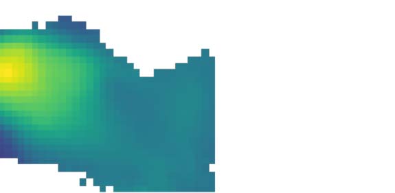
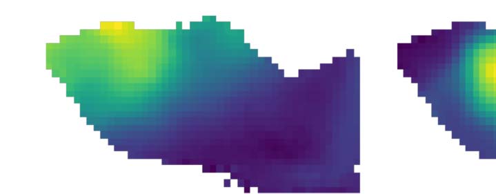
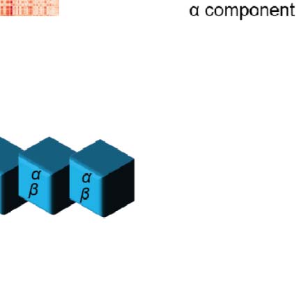
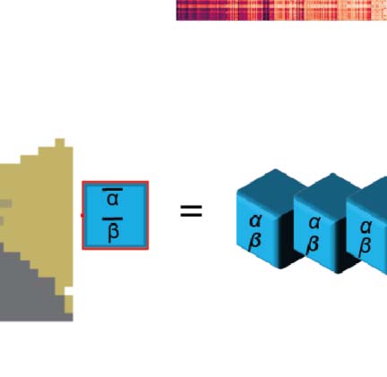
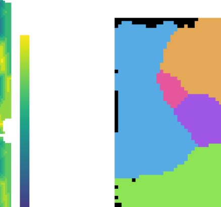
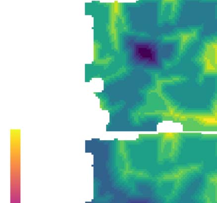
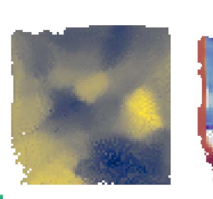
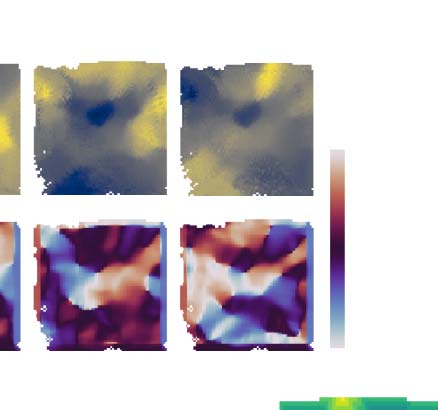
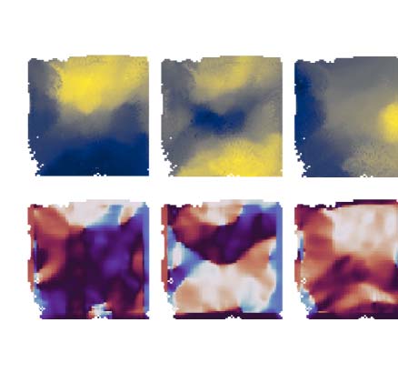
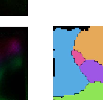
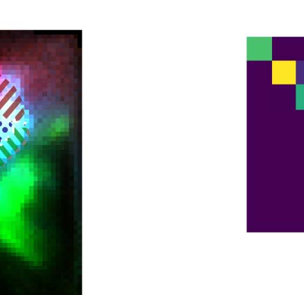
Figure 1. Parcellation at gradient reversals. (A) Horizontal and vertical retinotopy of mouse visual regions as measured by Garrett et al.
(2014). Data digitized from the original publication. (B) Gradients of the retinotopies (black arrows). Overlaid are regions with positive sign
(smallest rotation from horizontal to vertical gradient is clockwise, red) and with negative sign (smallest rotation is counterclockwise, blue).
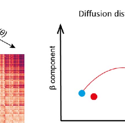
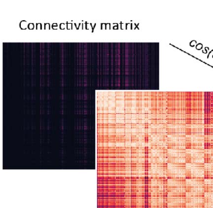
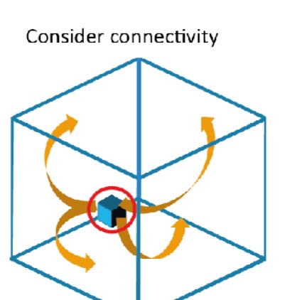
Green arrows denote examples of switches of the sign by a sudden reversal of one gradient. (C) Diffusion embedding. Build a similarity matrix
based on the connectivity strength of considered voxels and run diffusion process on this matrix to extract the embedded geometrical space of
connectivity. Extract then the first two dominant eigenvectors of the diffusion distance indicating the connectivity “profile” of the voxels. (D)
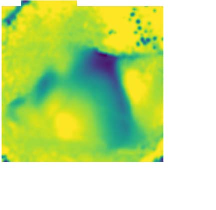
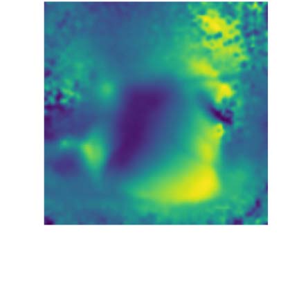
Left: Flattened view of mouse visual cortex. Subregions according to AIBS CCF are indicated in different colors. Right: For each pixel of the flat
view we average the first two diffusion coordinates (α and β) of the voxels mapping into the pixel. (E) Resulting mean α and β. (F) Gradients of
the mean α (top) and β (bottom). Red lines indicate manually annotated borders drawn at gradient reversals.
f
b
y
g
u
e
s
t
t
o
n
0
7
S
e
p
e
m
b
e
r
2
0
2
3
principle of gradient reversal might be useful to distinguish not merely sensory regions of the
same modality, but also different modalities and even sensory regions from nonsensory asso-
ciative areas.
RESULTS
Gradient Reversals in Visual Regions
To test our hypothetical approach, we first investigated whether the well-established gradient
reversals in visual cortices can be recreated from the voxelized connectivity. To that end, we
Network Neuroscience
1002
Connectivity-based parcellation
Flat map:
A general method that projects a
brain volume into two dimensions
while keeping spatial continuity.
gave the output of the diffusion embedding a spatial context that could be used to determine its
gradients. We used a flat map of mouse cortical regions that associates each connectivity voxel
with a discrete location in a two-dimensional grid. The projection preserves the relative area of
the surface defined by the layer 4 to layer 5 boundary. Voxels along an axis orthogonal to cor-
tical layers were mapped to the same location that we refer to as a pixel. At a voxel resolution of
100 μm, 13 ± 8 (mean ± SD) voxels were mapped to the same pixel. For each pixel, we con-
sidered the mean values of the diffusion embedding coordinates of the voxels mapped to that
pixel (Figure 1D). We could then calculate the gradient of any diffusion embedding coordinate
along the x- and y-axis of the pixelized image of isocortex (Figure 1E, F).
This approach explicitly “flattened away” the cortical layers, and it is known that the laminar
structure decidedly shapes connectivity (Felleman & Van Essen, 1991). However, we were
interested in a parcellation orthogonal to layer boundaries, similar to existing parcellations
and in accordance with the theory of the cortical column, that is, a piece of cortex spanning
all layers acting as a functional unit. We characterized the amount of information lost through
averaging by comparing the spread of diffusion embedding coordinates of voxels mapped to the
same pixel to the one over the mean values of pixels in the same region (Supporting Information
Figure S2). We found that the standard deviation of values within a pixel was almost two orders
of magnitude below the standard deviation over a region, demonstrating that the connectivity
profiles of voxels along a cortical column are likely similar, thus avoiding too much information
through flattening. Yet, in the future our algorithms might be extended by additionally con-
sidering a third gradient of a diffusion embedding coordinate along the depth-axis.
We applied this approach to the voxels associated with visual areas in the Allen Institute
Common Coordinate Framework (AIBS CCF; Wang et al., 2020; atlas.brain-map.org;
Figure 1D–F). We found in the two strongest components (from here on called α and β) several
gradient reversals that roughly coincide with the established parcellation. In the α component
we found reversals at the border between VISam and VISpm, splitting VISrl from VISa and VISal,
and a number of reversals splitting VISal, VISl, and VISli from the rest. In the β component we
found a local maximum, leading to a reversal when crossed in any direction, at the point
where VISp, VISpm, VISam, VISa, and VISrl meet. Additionally, reversals split VISa, VISrl,
and VISal from the rest. Crucially, the large area of the primary visual cortex ( VISp) was not
split up by reversals, instead depicting a continuous mapping characterized by only smooth
changes in the direction of both the α and β gradients.
We conclude that the diffusion embedding coordinates of voxelized connectivity contain
similar gradients and gradient reversals as the functional data based on neuron activity. As
such, it may be possible to build a parcellation based on it.
Context-Dependence of Connectivity Gradients
The diffusion embedding process yields connectivity trends ordered by their strengths. This
means that the results are potentially dependent on the context, that is, on which parts of cor-
tex were subjected to diffusion embedding together. A large-scale connectivity trend, spanning
the entire isocortex, such as the one described by component α in Supporting Information
Figure S3A, will not depict its full range of values when evaluated over a small patch. Conse-
quently it will appear weaker and may even be lost to noise. Conversely, a trend with a higher
spatial frequency would be less affected. This indicates that also reversals may appear or dis-
appear depending on the spatial context and scale.
We evaluated the degree of context-dependence by considering the gradients of the two
strongest components in an exemplary region (SSp-ll, the lower limb region of primary
Network Neuroscience
1003
l
D
o
w
n
o
a
d
e
d
f
r
o
m
h
t
t
p
:
/
/
d
i
r
e
c
t
.
m
i
t
.
t
/
/
e
d
u
n
e
n
a
r
t
i
c
e
–
p
d
l
f
/
/
/
/
/
7
3
9
9
9
2
1
5
4
8
3
6
n
e
n
_
a
_
0
0
3
1
2
p
d
t
.
f
b
y
g
u
e
s
t
t
o
n
0
7
S
e
p
e
m
b
e
r
2
0
2
3
Connectivity-based parcellation
Cosine distance:
A measurement of the angle between
pairs of vectors, here used to
evaluate similarity of connectivity
gradients.
somatosensory cortex) in different contexts: as part of the entire isocortex (Supporting Informa-
tion Figure S3A), the somatosensory and motor areas (same figure, panel B), somatosensory
areas (panel C), and individually (D). Note that the values of α and β are in arbitrary units
and consequently their sign is arbitrary as well. This means that only the orientations of gra-
dients and locations of reversals are meaningful, but not their direction. As such, results from
the level of isocortex down to somatosensory areas are very similar, only once SSp-ll is con-
sidered in isolation does β form a second, orthogonal gradient.
The emergence of an orthogonal gradient can be intuitively understood as follows: With the
region considered in isolation, we can assume that gradients related to region differences will
appear weak or not at all. As such, the strongest gradients would be related to the local connec-
tivity. Its known distance dependence (Holmgren, Harkany, Svennenfors, & Zilberter, 2003; Lübke,
Roth, Feldmeyer, & Sakmann, 2003; Perin, Berger, & Markram, 2011; Petersen & Sakmann, 2000)
will then result in gradients that simply reflect the spatial locations of the voxel. In the flat view, this
would result in two continuous (i.e., nonreversing) and orthogonal gradients, as observed.
We conclude that the orthogonality and continuity of the top two gradients, evaluated in a
region in isolation, may be an indicator that the region is atomic, that is, does not require fur-
ther subdivision. Later, we will further test this hypothesis in a model with a known set of
atomic regions. We defined two metrics that measure this trend: Gradient deviation, gd, eval-
uates how much the angle between the two strongest gradients deviates from 90 degrees, and
reversal index, ri, evaluates the absence of reversals by counting the pairs of pixels with an
angle above 90 degrees in the same component (for details, see Methods).
For SSp-ll we found that gd decreases significantly over scales (Supporting Information
Figure S3E), as expected. While ri is actually lowest at the scale of somatosensory areas and
increases slightly for SSp-ll in isolation, the reduction relative to the entire isocortex is still
substantial. Going forward, we will use these metrics to evaluate how distant a proposed
parcellation is from the theoretically derived ideal.
Evaluation of an Algorithmic Detection of Reversals
We implemented and executed two approaches to automatically split regions based on
connectivity gradients: cosine distance clustering and reversal detection (Figure 2). The first
generalizes the process of Campello, Moulavi, and Sander (2013) by considering the angle
between a pair of gradients, then clustering them based on similarity, using their cosine
distance. The second one explicitly determines pixels of the flattened view where a gradient
reverses (border pixels), then calculates for each pair of pixels the number of border pixels
separating them and clusters the resulting distance matrix (for details, see Methods).
Both approaches had their advantages and disadvantages. Reversal detection considered
only one component at a time, requiring the selection heuristic. Also, its convolution step left
a number of pixels at the borders of the region unlabeled (Figure 2, top right). Cosine distance
clustering, while considering several components together, did not explicitly seek out rever-
sals, but rather considered absolute differences in gradients. Results also tended to be noisier,
and it potentially left a number of pixels classified as outliers and thus unlabeled (Figure 2,
bottom right). These issues were addressed in a post-processing step that generalized region
assignment to unlabeled pixels and ensured that the resulting regions were spatially continu-
ous (see Supporting Information Figure S6; Methods).
As gradients and their reversals were context-dependent (see above), we did not stop after a
single application, but repeated the process recursively on the resulting subregions. This would
Network Neuroscience
1004
l
D
o
w
n
o
a
d
e
d
f
r
o
m
h
t
t
p
:
/
/
d
i
r
e
c
t
.
m
i
t
.
/
/
t
e
d
u
n
e
n
a
r
t
i
c
e
–
p
d
l
f
/
/
/
/
/
7
3
9
9
9
2
1
5
4
8
3
6
n
e
n
_
a
_
0
0
3
1
2
p
d
.
t
f
b
y
g
u
e
s
t
t
o
n
0
7
S
e
p
e
m
b
e
r
2
0
2
3
Connectivity-based parcellation
Figure 2. Automatic parcellation methods. Symbolic illustration of the workflow. Input is the matrix of connection strengths between voxels of
the region to parcellate. The 20 strongest components are extracted through diffusion embedding and gradients are calculated in a flattened
view (four gradients indicated). An initial parcellation is derived with one of two methods. Top: A gradient is selected, based on minimizing the
reversal index of the resulting parcellation, and a border map is built by convolving the normalized gradient with a uniform kernel. Pixels where
the length of the convolved gradient is below 0.97 are classified as border. Distance between a pair of pixels is calculated as the number of
border pixels on the path between them using the Dijkstra algorithm. An initial parcellation is generated through Ward linkage. Bottom: For each
gradient, pairwise cosine distances of the direction of the gradient are calculated. They are summed with weights corresponding to the strength
of the respective gradient. An initial parcellation is generated by the HDBSCAN algorithm. Finally, the initial parcellation is post-processed.
result in additional subdivisions, if new reversals appear at the reduced spatial scale. Further
repetitions thereby lead to not only a more fine-grained parcellation, but also a proposed
hierarchy of regions.
We evaluated this workflow against toy models of connectivity with a known, ground truth
parcellation. The purpose was to better understand how robustly the procedure works on con-
nectivity data with various interacting gradients. The models were built based on strong
assumptions about the organization of connectivity gradients. We do not claim that they reflect
biology, only that they are useful for evaluating the ability of our algorithms to detect known
gradients and their resistance against noise. We began with two very simplified models, revers-
ing hierarchy and node distance. Both hierarchically split the unit cube along orthogonal axes
into equally sized subregions, explicitly assign target gradients that reverse at the borders, and
assign connection strengths reflecting the gradient (Supporting Information Figure S4A). They
differed in the way the prescribed region hierarchy was taken into account (Supporting Infor-
mation Figure S4B1 vs. B2; for details, see Methods).
We attempted to recreate the parcellations of toy models with three hierarchy levels
(Figure 3A) and white noise at low (ϕ = 0.1) or high (ϕ = 5.0) amplitudes added to each weight
(Supporting Information Figure S4C; noise amplitude specified relative to the strength of the
signal). For the reversing hierarchy model at low noise, two successive applications of cosine
distance clustering or four applications of reversal detection recreated most of the parcellation,
although not at full granularity in the case of cosine distance clustering (Figure 3B1, Supporting
Information Figure S5 for results of intermediate steps). Under high noise conditions, only the
parcellation up to the second hierarchy level was recovered.
Conversely, for the node distance model, the full parcellation was reconstructed after a
single split in the low noise condition (Figure 3B2). Under the high noise condition, reversal
detection required two applications, and the output of cosine distance clustering did not
reflect the true parcellation in any way.
Network Neuroscience
1005
l
D
o
w
n
o
a
d
e
d
f
r
o
m
h
t
t
p
:
/
/
d
i
r
e
c
t
.
m
i
t
.
/
t
/
e
d
u
n
e
n
a
r
t
i
c
e
–
p
d
l
f
/
/
/
/
/
7
3
9
9
9
2
1
5
4
8
3
6
n
e
n
_
a
_
0
0
3
1
2
p
d
.
t
f
b
y
g
u
e
s
t
t
o
n
0
7
S
e
p
e
m
b
e
r
2
0
2
3
Connectivity-based parcellation
l
D
o
w
n
o
a
d
e
d
f
r
o
m
h
t
t
p
:
/
/
d
i
r
e
c
t
.
m
i
t
.
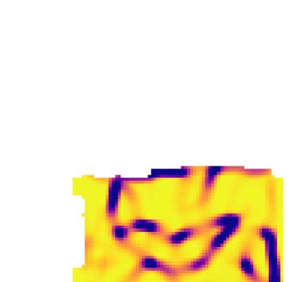
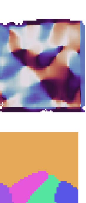
Figure 3. Applying splitting methods to toy models with known ground truth. Toy models of connectivity were constructed as in Figure 2. (A)
Reversing hierarchy and node distance models split the unit cube into equal quadrants. (B1) Left: Results of splitting the reversing hierarchy
model using reversal detection, with noise amplitudes ϕ = 0.1 (top) and ϕ = 5 (bottom). The number of applications of the splitting algorithm
before the solution converges is indicated above each result. Right: Splitting with cosine distance clustering. (B2) Same, for the node distance
model. (C) Gradient deviation and reversal index of the final output for the different approaches. Shades of red: Using cosine distance clus-
tering at low or high noise levels. Shades of blue: Using reversal detection. Bars and error bars indicate mean and standard deviation over
detected regions. (D) The random split model splits the volume at randomly drawn lines, connecting points on opposite sides with each other.
Exemplary random instance indicated. (E) Results for the exemplary instance in D. Left: After three splits with reversal detection. Right: After
following reversal detection with two splits using cosine distance clustering. (F) Uncertainty coefficient (uc) of the true parcellation and the
solution reached by the algorithms for three toy model instances. The instance in E is indicated in orange. Gray bars and error bars indicate
mean uc and its standard deviation for random control parcellations with the same numbers of regions. (G) Reversal index (left) and gradient
deviation (right) after successive splits for three instances.
t
/
/
e
d
u
n
e
n
a
r
t
i
c
e
–
p
d
l
f
/
/
/
/
/
7
3
9
9
9
2
1
5
4
8
3
6
n
e
n
_
a
_
0
0
3
1
2
p
d
.
t
f
b
y
g
u
e
s
t
t
o
n
0
7
S
e
p
e
m
b
e
r
2
0
2
3
We conclude that our methods are likely to recreate at least part of a parcellation, and that
resistance of the method against noise depends on the underlying architecture of connectivity,
which still remains unknown. Further, the ways in which the algorithm can fail is by yielding
an incomplete parcellation, or a completely incorrect parcellation. However, note that the
more severe second mode of failure was detectable through the quality metrics. Both ri and
gd of the results were higher for the incorrect solution than for the correct ones. Especially ri
appeared to be a good evaluator, yielding a value over two times (0.87 vs. 0.39) higher in the
case of the incorrect solution (Figure 3C). For the combination of reversal detection in the
reversing hierarchy model under high noise conditions, the recovered parcellation was incom-
plete in some parts and complete in others; this was reflected by a large standard deviation of
values of ri.
We evaluated to what degree the above generalizes to less idealized conditions in a more
complex model that generates random, more irregularly shaped subregions with different sizes
(Supporting Information Figure S4D; see Methods). We evaluated it at an intermediate noise
level of ϕ = 0.5 (Supporting Information Figure S4E). Based on our experiences with the sim-
pler models, we began with applications of the more conservative reversal detection until it
recovered no further granularity (Figure 3E, left), followed by cosine distance clustering for
further granularity (Figure 3E, right). Values of the reversal index and gradient deviation were
Network Neuroscience
1006
Connectivity-based parcellation
Uncertainty coefficient:
An information theoretical
measurement of statistical
dependence between random
variables, here used to measure
similarity of parcellations.
lowered at each split to around 0.2 and 20 degrees respectively (Figure 3G). Similarity of the
results and the true parcellation, measured by their uncertainty coefficient was high (Figure 3F),
yet the results were imperfect in two ways: Some borders were slightly shifted, and some sep-
arate subregions were merged into one.
Applying the Algorithms to Mouse Cortical Connectivity
We finally applied the splitting algorithm to the connectivity of the entire mouse isocortex. In
all of the six strongest components, except for the first and third, a prominent reversal was
immediately visible, spanning horizontally across the flat view (Figure 4A). We applied a first
split using reversal detection, as its results appeared more robust during our evaluations. The
method identified the sixth component as the one to use to minimize the result ri. This com-
ponent had 37% of the strengths of the first, strongest component (Figure 4B).
Closer inspection of the reversals of that component (Figure 4A2) and comparing with an
established parcellation revealed several strong reversals. This included one starting between
the prefrontal and anterolateral regions (Figure 4A2, red arrow), cutting through somatomotor
regions, and ending at the point where anterolateral, somatomotor, and temporal regions meet
(green arrow). This led to borders being detected that surround compact regions within the
somatomotor areas, as well as within temporal areas, and between medial and visual areas
(Figure 4C). In the distance metric calculated from the result, several compact regions with
low pairwise distance emerged (Figure 4D).
l
D
o
w
n
o
a
d
e
d
f
r
o
m
h
t
t
p
:
/
/
d
i
r
e
c
t
.
m
i
t
.
/
/
t
e
d
u
n
e
n
a
r
t
i
c
e
–
p
d
l
f
/
/
/
/
/
7
3
9
9
9
2
1
5
4
8
3
6
n
e
n
_
a
_
0
0
3
1
2
p
d
.
t
f
b
y
g
u
e
s
t
t
o
n
0
7
S
e
p
e
m
b
e
r
2
0
2
3
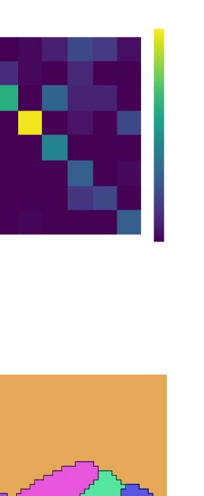
First split of isocortex into subregions. (A1) Top: Raw values of the first five diffusion components of mouse isocortex. Bottom: Angle
Figure 4.
of the gradient at each location. (A2) Left/right as A1 top/bottom for the sixth component that was selected for the split. Overlaid in black, left:
Gradient field, with each vector normalized to unit length. Right: Established rough parcellation (modules of J. A. Harris et al. [2019], but with
MOs and SSs separated). (B) Strengths of components relative to the strongest. Orange: The selected sixth component has a strength 37% of the
top one. (C) Lengths of vectors resulting from convolving the field in A2 with a two-dimensional Gaussian kernel with a width of five pixels.
Purple outlines: Pixels with a vector length <0.97, thus classified as a potential border. (D) Resulting distance metric; drawn is the distance
between any pixel and for two exemplary pixels indicated by red dots. (E) Resulting first split (colored areas), with established parcellation
overlaid and labeled.
Network Neuroscience
1007
Connectivity-based parcellation
The result (Figure 4E) led to eight subregions, where four of them covered the majority of
the prefrontal, medial, anterolateral, and visual modules of J. A. Harris et al. (2019), respec-
tively. However, they also contained significant parts of the temporal module, and the somato-
sensory and motor areas. Consequently, the remaining four subregions covered only a small
“core” of the MOs, primary somatomotor, SSs, and temporal regions, respectively. More for-
mally, we calculated the intersection-over-union of the established parcellation indicated in
Figure 4E with the regions resulting from the split at reversals (Figure 5B). We used the result
to assign tentative names to the regions (Figure 5C).
Curiously, the primary somatomotor regions were split up between six of the eight subre-
gions detected from reversals (Figure 4E). The apparent lack of such a fundamental level of
organization as clearly delineated somatomotor regions led us to investigate more closely.
First, we found that the split of somatosensory areas between five reversal-based regions
closely mirrors the split into regions associated with body parts of the established parcellation
(Supporting Information Figure S7A vs. B). The intersections with our anterolateral, SSp-core,
and SSs-core regions correspond to the mouth-, nose-, and upper limb-related parts, respectively.
The intersection with our visual regions corresponds to the barrel field, and medial regions to a
combination of lower limb and trunk-related parts. We conclude that reversal detection recreates
the internal parcellation of somatosensory regions, but not its external borders.
Another notable result was the split of the MOs and SSs regions of the established parcella-
tion into three subregions: located anterior, central, and posterior, respectively. We investi-
gated the incoming and outgoing connectivities of these subregions, considering whether
l
D
o
w
n
o
a
d
e
d
f
r
o
m
h
t
t
p
:
/
/
d
i
r
e
c
t
.
m
i
t
.
t
/
/
e
d
u
n
e
n
a
r
t
i
c
e
-
p
d
l
f
/
/
/
/
/
7
3
9
9
9
2
1
5
4
8
3
6
n
e
n
_
a
_
0
0
3
1
2
p
d
t
.
f
b
y
g
u
e
s
t
t
o
n
0
7
S
e
p
e
m
b
e
r
2
0
2
3
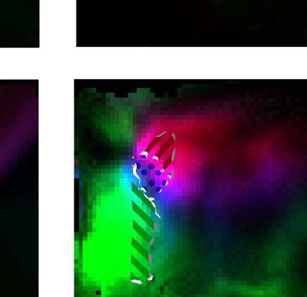
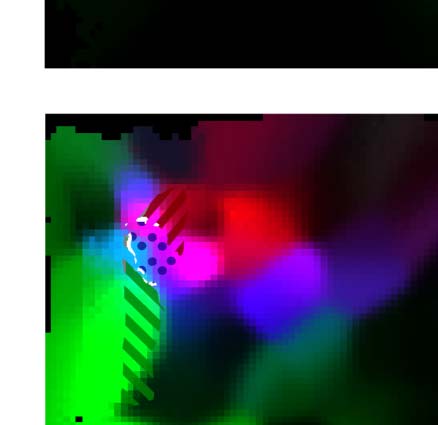
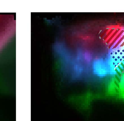
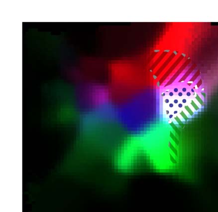
Figure 5. Evaluating the first split against the established parcellation. (A) Locations of afferent (left) and efferent (right) cortical locations of
regions in the established parcellation, when intersected with our parcellation. Gray lines: Established split into primary and secondary
somatosensory and motor regions. White lines: Proposed parcellation of our first split. Top: Region SSs is split into an anterior (red stripes),
core (blue dots), and posterior (green stripes) part by our parcellation. Afferent/efferent locations are indicated in red, blue, and green, respec-
tively. Bottom: MOs is similarly split into three parts. (B) Intersection over union of regions resulting from our first, reversal-based split (vertical)
and the established parcellation as indicated in Figure 4E. (C) Tentative labels for the resulting regions.
Network Neuroscience
1008
Connectivity-based parcellation
there is a fundamental difference in their organization, or whether they are better described as
single homogeneous regions (Figure 5A).
Unsurprisingly, each subregion interacted more strongly with its direct neighbors, but there
were also fundamental differences in their long-range connectivity. While the anterior part of
SSs receives its strongest inputs from anterior neighbors, the posterior part samples from medial
neighbors (specifically, from the barrel field in the established parcellation). While the poste-
rior part of MOs sends and receives extensive connectivity from prefrontal and medial areas,
largely avoiding somatosensory regions, the anterior part interacts mostly with the anterior
parts of primary motor and somatosensory regions. The core parts of both regions interacted
mostly with each other and the core parts of primary somatosensory regions; this was mostly
visible in the efferents of SSs.
Finally, the split of motor regions into subregions is arguably consistent with functional
data: Guo et al. (2014) described a role of specifically the anterolateral motor areas (ALM)
in an object location discrimination task that is not shared by the remaining parts of the motor
regions. The ALM region aligns closely with the intersection of motor areas and the reversal-
based anterolateral region.
Building a Hierarchy of Mouse Cortical Regions
We continued the applications of the algorithm to detect successive splits and thereby build a
hierarchy of regions. We performed a second application of reversal detection, followed by
three applications of cosine distance clustering. As before, we switched methods when reversal
detection no longer resolved additional granularity. In the following paragraphs we will
describe the result and the reasons to stop after five applications of the algorithm.
The resulting hierarchy has 41 leaf regions at six levels (Figure 6A1). Leaf regions exist at
each hierarchy level except for the root, indicating that these regions could not be split further
by the algorithms. The sizes of leaf regions vary considerably, with the largest one being
approximately eight times larger than the smallest (Figure 6A2).
l
D
o
w
n
o
a
d
e
d
f
r
o
m
h
t
t
p
:
/
/
d
i
r
e
c
t
.
m
i
t
.
t
/
/
e
d
u
n
e
n
a
r
t
i
c
e
-
p
d
l
f
/
/
/
/
/
7
3
9
9
9
2
1
5
4
8
3
6
n
e
n
_
a
_
0
0
3
1
2
p
d
.
t
Modularity:
A measurement that evaluates to
what degree connectivity in a given
parcellation is restricted within its
subregions.
We calculated at each hierarchy level the modularity of the parcellation (see Methods) with
respect to the raw connectivity strengths and compared them with corresponding values for
the established AIBS CCF hierarchy and parcellation (Figure 6B, left). As modularity naturally
decreases with increasing granularity, we plotted the results against the number of regions and
compared them also with 100 random, but spatially continuous, parcellations (see Methods;
Figure 6B, black line and error bars). For both reversal-based and established schemes the
modularity is significantly larger than in the random controls, but gets closer to them in the
lower hierarchy levels. When we calculated modularity based on the (cosine) similarity of
connectivity instead, results were comparable (Figure 6B, right).
f
b
y
g
u
e
s
t
t
o
n
0
7
S
e
p
e
m
b
e
r
2
0
2
3
Note that neither scheme aims to maximize the measure. The AIBS scheme unifies multiple
historical schemes based on anatomy and neuron function, and our scheme allows very dif-
ferent connectivity within a subregion as long as it varies along a continuous gradient. Yet, this
measure shows that our parcellation provides a qualitatively similar solution. This was also
evident in a visual comparison of the connectivity matrices (Supporting Information Figure S7C).
Further note that to ensure comparability, we calculated modularity in the flattened view also for
the AIBS parcellation; values may differ if calculated between the original voxels.
The demonstrated qualitative similarity between the reversal-based and the established
solutions led to the question to what degree they actually describe the same parcellation.
To quantify this, we calculated their similarity in terms of the uncertainty coefficient (Figure 6C;
Network Neuroscience
1009
Connectivity-based parcellation
l
D
o
w
n
o
a
d
e
d
f
r
o
m
h
t
t
p
:
/
/
d
i
r
e
c
t
.
m
i
t
.
t
/
/
e
d
u
n
e
n
a
r
t
i
c
e
-
p
d
l
f
/
/
/
/
/
7
3
9
9
9
2
1
5
4
8
3
6
n
e
n
_
a
_
0
0
3
1
2
p
d
t
.
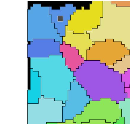
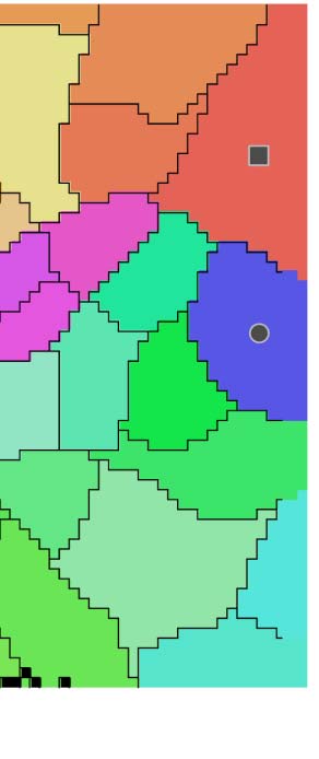
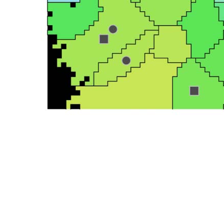
Figure 6. Complete parcellation results. (A1) Tree plot of the resulting hierarchy after five successive splits (top to bottom). Size of leaf nodes
is proportional to region size. (A2) Locations of leaf regions. Colors as in A1. (B) Modularity of parcellations evaluated with the voxelized
connectivity matrix (left) or matrix of similarity of connectivity (right). Plotted against the number of regions at each hierarchy level for the
reversal-based parcellation (blue/green), a random parcellation (see Methods) with the same number of regions (black/gray), and the AIBS CCF
parcellation (red/yellow). (C) Similarity of the AIBS CCF parcellation and the reversal-based parcellation, measured as their uncertainty coef-
ficient (see Methods). Blue bars: Values at various hierarchy levels. Black dots and gray error bars: For a random parcellation with the same
number of regions instead. (D) Values of gd (D1) and ri (D2) indicated by the color of nodes in tree plots of the hierarchy. Red indicates values
above the acceptance threshold, orange if it is an internal node. Insets: Box plots of the values after each split and the changes caused by
individual splits (gray lines).
f
b
y
g
u
e
s
t
t
o
n
0
7
S
e
p
e
m
b
e
r
2
0
2
3
for details see Methods). This information theoretical measure yields values between 0 and 1,
with 1 indicating a parcellation identical to the established one and values close to 0 a par-
cellation orthogonal to it, such as the split into cortical layers. As any split into subregions is
likely to produce values larger than 0, we compared the results with the same random parcel-
lations as before. We found that values for the reversal-based parcellation were significantly
lower than for the controls; that is, it is actually more orthogonal to the established scheme
than expected by chance. This indicates that differences between the schemes are due to the
reversal method detecting previously unaccounted trends in connectivity and are not merely
generating random results or picking up noise. However, the trend weakened with number of
Network Neuroscience
1010
Connectivity-based parcellation
regions, until after five splits the reversal-based solution was within a single standard deviation
of the controls with respect to this measurement.
As a final test, we evaluated how the reversal-based parcellation evolves with each split
with respect to the previously defined quality metrics (Figure 6D). We found a large spread
of values for both metrics, but the overall mean and median decreases reliably with each split.
Occasionally, a child region results in a larger value for a metric than its parent, indicating a
worse solution, but this is typically followed by an even larger decrease in the next split
(Figure 6D, inset, gray lines). Yet, after five splits, three regions were above the defined threshold
for gd (Figure 6D1, red; A2, circles), and four for ri (Figure 6D2, red; A2, squares). All of them
appeared before the last split, indicating that the algorithm was not capable of splitting them
further, and that additional applications would not lead to an improvement.
We decided to stop after five applications of the algorithm for a combination of reasons:
First, at that point the parcellation was close to a random parcellation in terms of modularity
and uncertainty coefficient (Figure 6B, C). Second, the number of new regions resulting from
the split had stagnated with most regions already being “atomic.” Third, remaining regions
with values for gd and ri exceeding the threshold could not be split by the algorithm.
l
D
o
w
n
o
a
d
e
d
f
r
o
m
h
t
t
p
:
/
/
d
i
r
e
c
t
.
m
i
t
.
/
/
t
e
d
u
n
e
n
a
r
t
i
c
e
-
p
d
l
f
/
/
/
/
/
7
3
9
9
9
2
1
5
4
8
3
6
n
e
n
_
a
_
0
0
3
1
2
p
d
t
.
f
b
y
g
u
e
s
t
t
o
n
0
7
S
e
p
e
m
b
e
r
2
0
2
3
DISCUSSION
We have demonstrated that gradient reversals at the borders between adjacent sensory regions
can also be found in the connectivity of voxels belonging to the regions. We have further dem-
onstrated that these gradients can be isolated through the diffusion embedding technique. This
approach differs conceptually from previous approaches based on clustering of matrices of
connectivity similarity. Clustering-based approaches are based on the idea that connectivity
profiles of voxels within a region are homogeneous or at least similar. However, as pointed
out by Eickhoff et al. (2015), functional gradients often exist within regions, as shown in earlier
studies (Hensel et al., 2015; Wandell et al., 2007). As they are likely reflected by correspond-
ing connectivity gradients, this contradicts the underlying assumption of similarity clustering.
Conversely, our approach allows for dissimilar profiles, as long as the dissimilarity is the result
of a continuous gradient within the region, reversing at its border.
We have developed an algorithmic pipeline based on this approach that largely automat-
ically breaks up a voxelized connectivity structure into a partition of the volume into subre-
gions (reversal-based parcellation). In addition to the partition, the solution also provides a
tentative hierarchy of subregions, although evaluations on a test model show that individual
levels of the hierarchy may remain incomplete. At the same time, the evaluations demon-
strated a very large degree of robustness against unstructured noise in the input connectivity
data. We also developed quality metrics that can be used to detect algorithm failure. They can
also be applied to other parcellations to evaluate how close they come to an ideal reversal-
based solution.
At the core of the pipeline is the automatic placement of region border, which we imple-
mented with two different approaches. Of these, reversal detection was more conservative,
requiring more successive applications and not resolving the full granularity (Figure 3B1; Sup-
porting Information Figure S4C2). This was because it requires a subregion to be completely
encircled by reversals to be detected. Conversely, cosine distance clustering was more affected
by noise, especially when tasked to split large subvolumes (Figure 3B2). Therefore, we found
that the best approach combines the two, beginning with reversal detection until no further
granularity can be resolved, followed by cosine distance clustering. Both approaches are
Network Neuroscience
1011
Connectivity-based parcellation
limited in terms of spatial resolution by the numerical calculation of a spatial gradient. This
makes it harder to resolve narrow and elongated-shaped regions. Regions narrower than three
times the voxel resolution are theoretically impossible to resolve, and in practice the limit is
even higher.
Beyond these algorithmic issues, one potential danger lies in the hierarchical nature of the
algorithm combined with the context dependence of the detected gradients. This means that
great importance is given to the first few splits of the target volume, as they determine the
context used for all future splits. Should the algorithms fail in the early steps, the entire par-
cellation would be affected. Other algorithms fail less drastically, with errors at one location
not necessarily affecting others.
Finally, one limitation of the presented approach is that it requires a way to project voxel
positions into the plane, with the resulting parcellation always being orthogonal to the projec-
tion. This does not readily generalize to all brain structures. Mathematically, all techniques we
employed could be generalized to work in three dimensions instead, allowing their use in
regions where a flattening is harder to define. Cosine distance clustering can be expected to
work in three dimensions as well, while it remains unclear whether detected reversals would
encircle subregions also in three dimensions.
l
D
o
w
n
o
a
d
e
d
f
r
o
m
h
t
t
p
:
/
/
d
i
r
e
c
t
.
m
i
t
.
t
/
/
e
d
u
n
e
n
a
r
t
i
c
e
-
p
d
l
f
/
/
/
/
/
7
3
9
9
9
2
1
5
4
8
3
6
n
e
n
_
a
_
0
0
3
1
2
p
d
t
.
f
b
y
g
u
e
s
t
t
o
n
0
7
S
e
p
e
m
b
e
r
2
0
2
3
We applied the algorithms to the voxelized connectivity of mouse isocortex (Knox et al.,
2019; Oh et al., 2014). The resulting parcellation differed from established schemes, but did so
in a demonstrably nonrandom way. Further, when evaluated in terms of modularity, it was
further away from a random solution than the established scheme. This indicates that the
reversal-based parcellation captures novel connectivity trends that cannot be detected when
connectivity is evaluated with respect to the established parcellation. One example is a
specialization of the anterolateral motor regions that was not present in the established
parcellation, but had been described in earlier literature (Guo et al., 2014). This demonstrates
the importance of also considering a parcellation based on connectivity.
The parcellation presented is not to be understood as a replacement of existing schemes,
but as complementary. Which one is superior depends on the use case. For example,
approaches to connectivity-based parcellation that maximize modularity will by design yield
subregions with mostly internal connectivity. This is useful for identifying units that can be
described in isolation from the rest of the brain, for example in modeling. On the other hand,
our scheme is more useful in use cases that require continuous gradients in a region. For exam-
ple, mouse brain connectivity has been modeled using a single continuous topographical
mapping per pair of regions (Reimann et al., 2019). The presence of several reversing gradients
in the MOs and SSs regions of the AIBS CCF parcellation led to inaccuracies of the model.
Outside of specific applications, a parcellation is expected to reveal something about the
organization of the brain. As it is neuron function that we are trying to understand, an argu-
ment can be made in favor of function-based parcellation. On the other hand, connectivity as
one of the underlying causes of neuron function (van den Heuvel et al., 2015) puts it closer to
the root of the mechanisms we are trying to decipher. Here as well, both approaches can be
used in conjunction. For example, one can contrast function-based parcellation, where pri-
mary sensory areas are prominently separated with our results, that lacks such a delineation.
It is important to consider that the presented results were based on intracortical connectivity
only, while primary sensory areas are largely defined by their thalamic input sources (Sherman,
2016). As such, that aspect of the functional parcellation reflects the quality of bottom-up
inputs, and our results are more aligned with the structure of intracortical processing. By con-
sidering both, we can improve our understanding of the structure-function relation.
Network Neuroscience
1012
Connectivity-based parcellation
Network Neuroscience
In this context, one advantage of our approach is its adaptability with respect to the types of
connectivity to be considered. It would be possible to generate a parcellation based on
thalamocortical inputs that we predict to feature primary sensory areas prominently. Using
corticofugal connectivity and comparing the results may reveal even more aspects (Usrey &
Sherman, 2019). Yet, even with only intracortical connectivity considered, our result is useful
for understanding the organization of mouse intracortical connectivity. This can be in the form
of analyzing large-scale in vivo recordings of neuronal activity with respect to our parcellation
to test which aspects of neuronal function are aligned with it.
The adaptability of the approach extends to the use of other data sources. The set of
algorithms can be readily applied to any source of voxelized connectivity in any organism,
including undirected connectivity, such as functional connectomes. Indeed, comparable
gradients have been found in human functional connectivity data (Katsumi et al., 2021). As
functional connectivity can be derived for single individuals, our technique could be used for
assessing interindividual differences, or changes resulting from disease and injury. Derived
parcellations come with a distance metric in the form of the uncertainty coefficient, and
differences could be easily interpreted in the form of, for example, growth and shrinkage of
corresponding regions. In fact, the algorithms can be easily adapted to data outside of connec-
tivity, working with any voxelized data source where similarity of pairs of voxels can be
defined and calculated. This encompasses for example gene expression data, although it is
unclear whether these data are organized around spatial gradients with reversals.
Simultaneously a strength and a weakness of the results presented here are their provenance
from a single data source. This ensures a certain level of standardization across the entire cor-
tex. The splitting algorithms also treat each cortical location equally, leading to a result that
avoids the potential biases arising when different parts of the parcellation are based on different
sources and different techniques. On the other hand, the result will be affected by any bias or
weakness in the source data itself. This can be improved by combining several sources of con-
nectivity data or considering both anatomical and functional reversals simultaneously.
METHODS
Diffusion Embedding
In short, the method considers a diffusion process along the edges of a graph, described as a
Markov chain with a transition matrix determined by the normalized (cosine) similarity of
incoming and outgoing connectivity of each voxel. The embedding coordinates are then given
by the eigenvectors of the transition matrix, scaled by their eigenvalues.
Let C[i,j] be the strength of connectivity between brain voxels i and j, be the set of voxels in
the volume to be partitioned, the volume to be considered as a connectivity target, and n =
||. In this work, we considered intracortical connectivity exclusively, hence = , but other
options are possible, such as partitioning cortex based on its connectivity with thalamus.
The connectivity profile P of each voxel was then given by the concatenation of C with its
transpose, such that each row of the resulting n × 2n matrix corresponded to the incoming
and outgoing connectivity of a voxel in . P 0 was a normalized version of P and S the cosine
similarity of P 0:
P 0
½
i;j
(cid:2) ¼
P i;j
(cid:2)P
½
v¼0…nP i;v½
(cid:2)
;
S ¼ P 0P 0⊤:
(1)
(2)
1013
l
D
o
w
n
o
a
d
e
d
f
r
o
m
h
t
t
p
:
/
/
d
i
r
e
c
t
.
m
i
t
.
t
/
/
e
d
u
n
e
n
a
r
t
i
c
e
-
p
d
l
f
/
/
/
/
/
7
3
9
9
9
2
1
5
4
8
3
6
n
e
n
_
a
_
0
0
3
1
2
p
d
t
.
f
b
y
g
u
e
s
t
t
o
n
0
7
S
e
p
e
m
b
e
r
2
0
2
3
Connectivity-based parcellation
In a final normalization, each entry of S was scaled, based on the product of the sums of
values in the corresponding row and column as follows:
W ¼ D−0:5SD−0:5;
(3)
where D was a diagonal matrix with each entry D[i,i] being the sum of the corresponding row
of S. W was then used as the transition matrix, which with this last normalization
approximates the Fokker-Planck diffusion (Coifman & Lafon, 2006).
The embedding coordinates used were then the eigenvectors of W, scaled by their eigen-
values (λt; though we used exclusively t = 1). Coordinates were sorted by their eigenvalues and
the strongest ones considered as described in the rest of the manuscript. For the steps from
Equation 3 on, we used the implementation of github.com/satra/mapalign, as described in
Coifman and Lafon (2006) and Langs, Golland, and Ghosh (2015) with parameters α = 0.5
and t = 1.
Gradient Deviation and Reversal Index
We defined two quality metrics for proposed parcellations based on the gradients found within
each of their regions. First, gradient deviation, gd, evaluates the orthogonality of the two
strongest gradients in a region κ:
gdκ ¼
X
(cid:4)
(cid:4)
(cid:2)
λ αx;y ; βx;y
(cid:3)
(cid:4)
(cid:4);
− 90
(4)
where λ(., .) measures the angle between two gradients, here the two strongest gradients α, β at
pixel (x, y).
x;yð
Þ2κ
The second metric, reversal index, ri, evaluates the continuity of the gradients, that is, the
absence of reversals. It first counts the pairs of pixels with an angle above 90 degrees in the
same component ω:
(cid:4)
(cid:5)
(cid:4)
(cid:3)
(cid:3)
(cid:3)
(cid:2)
(cid:2)
2 κ; λ ωxi ;yi
; ωxj ;yj
(cid:4)
(cid:6)
(cid:4)
> 90
;
xi; yi; xj; yj
ð
: xi; yi
riω;κ ¼
(5)
(cid:2)
Þ 2 κ; xj; yj
2
Nκ
where Nκ refers to the number of pixels in κ. Then, this measurement is summed over the two
strongest components:
riκ ¼ riα;κ þ riβ;κ:
(6)
Algorithmic Detection of Reversals
Two approaches automatically detected gradient reversals and drew borders between regions
separated by them: cosine distance clustering and reversal detection.
Both begin by applying diffusion embedding (Vos de Wael et al., 2020) to the matrix of
directed connection strengths between voxels, extracting the 20 strongest components
(Figure 2, left). As discussed in the Introduction and Figure 1, we work in a flattened view
of the volume of interest; as such we average the value of each component over the voxels
mapped to the same pixel. We then calculate their gradients with respect to the grid of pixels.
The next steps differ between the two approaches.
Cosine distance clustering (Figure 2, bottom) considers the gradients of the strongest 20
components and directly calculated a distance metric based on them. For each pair of pixels,
a weighted sum of cosine similarities of the gradients was considered, where the weight was
equal to the strength of the associated component.
Network Neuroscience
1014
l
D
o
w
n
o
a
d
e
d
f
r
o
m
h
t
t
p
:
/
/
d
i
r
e
c
t
.
m
i
t
.
/
t
/
e
d
u
n
e
n
a
r
t
i
c
e
–
p
d
l
f
/
/
/
/
/
7
3
9
9
9
2
1
5
4
8
3
6
n
e
n
_
a
_
0
0
3
1
2
p
d
t
.
f
b
y
g
u
e
s
t
t
o
n
0
7
S
e
p
e
m
b
e
r
2
0
2
3
Connectivity-based parcellation
First the gradient of the nth component (ωn) at a location i was normalized (as in Figure 1F):
(cid:8)
(cid:7)
∇i
ωn
¼
Δωi
n
Δx
;
Δωi
n
Δy
; ∇^
ωn
i ¼
(cid:4)
(cid:4)
∇i
ωn
∇i
ωn
(cid:4)
(cid:4) :
(7)
(8)
Then the weighted sum of cosine similarities was calculated:
Si;j
ωn
¼
X20
n¼1
wn ⋅ ∇^
i ⋅ ∇^
j
ωn
ωn
:
This was then converted to a distance by subtracting the value from the maximum possible
value:
Di;j
ωn
¼
X20
n¼1
wn − Si;j
ωn
:
(9)
We then applied the HDBSCAN algorithm (Campello et al., 2013), resulting in a hierarchical
clustering that yields an initial parcellation.
Reversal detection (Figure 2, bottom) considered the normalized gradient of a single com-
, as above. We calculated the degree of reversal at each loca-
ponent in its flattened view, ∇^
ωn
tion by convolving the gradient field with a two-dimensional Gaussian kernel. If gradients
around a pixel have the same orientation, the vector resulting from the convolution at that
point will also have unit length; conversely, a reversal would lead to gradients with inverted
orientation cancelling each other out in the convolution. We considered a convolved vector
shorter than 0.97 to indicate that the location was part of a border. We then determined con-
tiguous regions encircled by the same boundary in the following way: We began by building a
graph where each node represented a pixel and edges were placed between all pairs of neigh-
boring pixels (direct or diagonal neighbors). The length of an edge was 1 if either of the pixels
was tagged as a border, and 0 otherwise. We calculated distances between all pixels as the
length of the shortest path in the graph between the pair, as calculated by the Dijkstra algo-
rithm (Dijkstra, 1959). Finally, we generated groups of pixels by running the Ward linkage
algorithm on the matrix of pairwise distances. We chose the number of clusters between 2
and 10 by optimizing the resulting silhouette score.
Unfortunately, reversals might not be observed equally on every diffusion component, so a
first operation is to determine which component to use to perform the reversal detection.
While an intuitive choice may be the first (i.e., strongest) component, in practice we found
that (a) this component was not guaranteed to yield the most useful split; and (b) the following
components often had very similar strengths, indicating that their order may be partially arbi-
trary. Consequently, we decided to run the algorithm on all of the 20 strongest components
and choose the one that minimizes the reversal index, ri, within the resulting subregions:
ω(cid:3) ¼ arg min
ω
P
κriω;κ
mω
;
(10)
l
D
o
w
n
o
a
d
e
d
f
r
o
m
h
t
t
p
:
/
/
d
i
r
e
c
t
.
m
i
t
.
/
/
t
e
d
u
n
e
n
a
r
t
i
c
e
–
p
d
l
f
/
/
/
/
/
7
3
9
9
9
2
1
5
4
8
3
6
n
e
n
_
a
_
0
0
3
1
2
p
d
.
t
f
b
y
g
u
e
s
t
t
o
n
0
7
S
e
p
e
m
b
e
r
2
0
2
3
where mω is the number of subregions resulting when a split is applied based on ω and ri is
defined as in Equation 5. Note that in actual biological data, the 20th component still had a
strength of 10% of the first component.
Post-Processing the Initial Split
The shortcomings of both methods required a number of post-processing steps (Supporting
Information Figure S6). First, unlabeled pixels (see above) needed to be classified. To that
Network Neuroscience
1015
Connectivity-based parcellation
end, we train a support vector machine to classify the unlabeled pixels based on their x and y
coordinates in the flat coordinate system (Supporting Information Figure S6A). This step serves
not only to extrapolate the first classification, but also to generalize the output to a less noisy
result. Indeed, because of potential noise in the input data, the resulting parcellation of the first
gradient classification can be irregular and scattered, especially for cosine distance clustering.
Second, at this stage all pixels are classified but some clusters of the same class can be spatially
noncontinuous; therefore, these clusters must be differentiated. This is done by hierarchical
clustering of pixels of the same class based on their Euclidean distance (Supporting Informa-
tion Figure S6B). Third, we “unflatten” the resulting parcellation from pixels to voxels by
looking up the reverse images of each pixel (Supporting Information Figure S6C). Finally,
we specify a minimum size threshold for the resulting regions to reject any regions that are
unrealistically small and merge them with their closest neighbor (Supporting Information
Figure S6D).
Building Toy Models of Connectivity
We built models of connectivity inside a voxelized 3D cube, with a regular grid of a given
resolution and depth specifying a spatially nested hierarchy of regions. Each level of the hier-
archy split the cube along one axis, alternating between the y- and z-axis (Supporting Infor-
mation Figure S4A). Connection strengths were generated for a hierarchy level by reversing the
diffusion process. We prescribed continuous and reversing target values of the two strongest
components, α and β, that is, attributing increasing—or decreasing—component values to
voxels and reversing these components where a different region starts (Supporting Information
Figure S4A, right). For example, for a split along the y-axis,
ð
α x; y; z
(cid:4)
(cid:4)
Þ ¼ 2 y ⋅ n
(cid:4)
2
j
− y ⋅ n
2
k
þ 0:5
(cid:4)
(cid:4)
ð
(cid:4); β x; y; z
Þ ¼ z;
(11)
where n is the resolution of the model, that is, the number of subregions in the hierarchy level.
The connection strength between each pair of voxels i and j was then defined based on
Euclidean distance of those values:
ð
S i; j
Þ ¼
q
ffiffiffiffiffiffiffiffiffiffiffiffiffiffiffiffiffiffiffiffiffiffiffiffiffiffiffiffiffiffiffiffiffiffiffiffiffiffiffiffiffiffiffiffiffiffiffiffiffiffiffiffiffiffiffiffiffiffiffiffiffiffiffiffiffiffiffiffiffiffiffiffiffiffiffiffiffiffiffiffiffiffiffiffiffiffiffiffiffiffiffiffiffiffiffiffiffiffiffiffiffiffiffiffiffiffiffiffiffiffiffiffiffiffiffiffiffi
(cid:2)
(cid:3)
2
ð
α xi; yi; zi
(cid:2)
Þ − β xj; yj; zj
(cid:2)
Þ − α xj; yj; zj
2 þ β xi; yi; zi
ð
(cid:3)
(cid:3)
(cid:2)
(cid:3)
ð
C i; j
Þ ¼ e
p
−
ffiffiffiffiffiffi
S i;jð
Þ
2⋅σ2
þ n ϕð Þ;
;
(12)
(13)
where σ was set to 0.1 times the maximum of S(x, y), and n(ϕ) denotes noise with a uniform
distribution between −ϕ and ϕ that was added to test the resistance against noise.
This process could be applied at a given level of the hierarchy to connect the subvolumes at
that level of the hierarchy (Supporting Information Figure S4A, right). This yielded one connec-
tion matrix per hierarchy level. We combined matrices for all hierarchy levels by piecewise
multiplication of their entries (reversing hierarchy model, Supporting Information Figure S4B1,
C1). As an alternative approach, we only considered the connection matrix for the lowest hier-
archy level. Then, for each entry we considered the pair of regions it corresponds to, looked up
their path distance in the hierarchy tree, and divided the value of the entry by that distance
(node distance model, Supporting Information Figure S4B2, C2).
We built more complex, random models (random split model ) based on recursively splitting
the volume at randomly drawn lines. For each split, first the angle of the line is randomly
drawn. It is drawn with uniform probability from [0, 2π] for the first split and from [α + π
−
2
0.5, α + π
2 + 0.5] for all following, where α is the angle of the previous split. The location of the
Network Neuroscience
1016
l
D
o
w
n
o
a
d
e
d
f
r
o
m
h
t
t
p
:
/
/
d
i
r
e
c
t
.
m
i
t
.
/
t
/
e
d
u
n
e
n
a
r
t
i
c
e
–
p
d
l
f
/
/
/
/
/
7
3
9
9
9
2
1
5
4
8
3
6
n
e
n
_
a
_
0
0
3
1
2
p
d
.
t
f
b
y
g
u
e
s
t
t
o
n
0
7
S
e
p
e
m
b
e
r
2
0
2
3
Connectivity-based parcellation
line is then randomly determined such that the subvolume is split between 40%–60% and
60%–40%. The process is repeated for each resulting subvolume until they are below a size
threshold, or until either a specified number of regions have been generated.
Connectivity was based on the location of each placed line. Each line defined a mirror
operation. Points mirrored on top of each other are then set to project to each other in the
following way: Let P, P 0 be a pair of points mirrored on top of each other. The strength of
connections from P is then given by
Sx;y ¼ Π ⋅ e
(cid:2)
ð
− D P
(cid:3)
Þ
þ1
;
(cid:2)
0 ; x;y½
ρ
(14)
where Π and ρ depended on the hierarchy level L of the split, beginning at 1 for the first split.
Π ¼
1
Þ
max 4 − L; 1
ð
;
ρ ¼ 25 ⋅ e
−L
3 :
(15)
(16)
l
D
o
w
n
o
a
d
e
d
f
r
o
m
h
t
t
p
:
/
/
d
i
r
e
c
t
.
m
i
t
.
Calculation of the Uncertainty Coefficient of Pairs of Parcellations
2 RX. We describe this association as
A parcellation X associates each voxel v with a region r X
i
i and NX = (cid:2)i nX
X(v) = i. Let nX
the total number of
voxels. We can then consider PX, the probability distribution given by the region associated
with a voxel that has been randomly picked (with uniform probabilities):
i be the number of voxels associated with r X
i
P X : pX
i
¼ nX
i
NX
:
As with any probability distribution, we can calculate its entropy:
(cid:3)
(cid:2)
H P X
¼ −
X
pX
i
(cid:2)
⋅ log pX
i
(cid:3)
:
i
(17)
(18)
Given two parcellations X, Y that are defined on the same set of voxels, we can similarly con-
sider their joint distribution P (X,Y ), where p X;Yð
i;jð
assigned to region i in X and to j in Y.
is the probability that a random voxel is
Þ
Þ
This allows us to calculate the mutual information of the probability distributions associated
with a pair of parcellations. This is the reduction of entropy of one of them when the value of
the other is revealed. That is, if you know the region identity of the random voxel according to
one parcellation, how much does it help you to guess its identity in the other?
/
/
t
e
d
u
n
e
n
a
r
t
i
c
e
–
p
d
l
f
/
/
/
/
/
7
3
9
9
9
2
1
5
4
8
3
6
n
e
n
_
a
_
0
0
3
1
2
p
d
t
.
f
b
y
g
u
e
s
t
t
o
n
0
7
S
e
p
e
m
b
e
r
2
0
2
3
(cid:2)
I P X ; P Y
(cid:3)
¼
X
X
p X;Yð
i;jð
Þ
i
j
Þ
⋅ log
0
@
Þ
p X;Yð
i;jð
Þ
⋅ pY
pX
j
i
1
A:
Normalizing it by the entropy of X yields the uncertainty coefficient:
(cid:2)
U P X ; P Y
(cid:3)
¼
(cid:2)
I P X ; P Y
Þ
H P Xð
(cid:3)
:
(19)
(20)
This is a measure of similarity between parcellations. Intuitively, if revealing that the identity
of a voxel according to Y is j yields a lot of information about its identity in X, this means there
must be at least one region in X that overlaps strongly with j. Mathematically, we can see how
Network Neuroscience
1017
Connectivity-based parcellation
for X = Y Equation 19 equals Equation 18 because p X;Yð
i;jð
i ≠ j. Consequently, in that case U(PX; PY) = 1.
Þ
Þ = pX
i = pY
j
for i = j and p X;Yð
i;jð
Þ
Þ = 0 for
Conversely, if PX and PY are statistically independent, then by definition P X;Yð
Þ
Þ = P X
i;jð
i
consequently I(PX; PY) = U(PX; PY) = 0. This is the case for orthogonal parcellations.
· P Y
j and
In the manuscript we set X to the established AIBS CCF parcellation and Y to whichever
parcellation or control parcellation we want to evaluate.
Calculation of the Modularity of a Parcellation
The modularity of a parcellation with respect to a matrix of connection strengths is the differ-
ence between the fraction of connection strength that is found between pairs of voxels in the
same region and the fraction of the number of pairs of voxels in the same region.
Let X be a parcellation as defined in the previous section. Let M be the connectivity matrix,
such that M(v, w) yields the strength of connectivity between voxels v and w. Then the fraction
of connection strength found within a region is
P
γ
M Xð Þ ¼
v;w:X vð Þ¼X wð
P
v;w M v; wð
ÞM v; wð
Þ
Þ
:
The fraction of voxel pairs that are in the same region, relative to all possible pairs, is
ϕ Xð Þ ¼
P
⋅ nX
inX
i
i
NX ⋅ NX
:
The modularity is then the difference between the two, γM(X ) − ϕ(X ). Individually their values
are between 0 and 1. This measurement is between −1 and 1.
If connectivity strengths are independent of the parcellation, then the expected value of the
measurement is 0; if strong connectivity is found predominately within a region, the measure-
ment is greater than 0.
Generation of Random Control Parcellations
We generated comparable but random parcellation schemes the following way: First, a ran-
dom control is paired with the reversal-based parcellation after a given number of splits in
order to match its number of resulting subregions. For a given number of subregions, we gen-
erated 100 random parcellations with two different algorithms (50 per algorithm).
First, we generated 50 schemes by first randomly distributing a number of points equal to
the target number of subregions within the axis-aligned bounding box of the pixel positions of
the flat view. Points were randomly picked with uniform density within the bounding box.
Then, pixels were classified into subregions based on the random point they were closest
to. Second, we generated 50 schemes according to the random split model described above.
Both controls generated random parcellations with spatially continuous subregions of various
sizes and the same number of subregions as the reversal-based parcellation.
ACKNOWLEDGMENTS
This study was supported by funding to the Blue Brain Project, a research center of the École
polytechnique fé dé rale de Lausanne (EPFL), from the Swiss government’s ETH Board of the
Swiss Federal Institutes of Technology.
Network Neuroscience
1018
(21)
(22)
l
D
o
w
n
o
a
d
e
d
f
r
o
m
h
t
t
p
:
/
/
d
i
r
e
c
t
.
m
i
t
.
t
/
/
e
d
u
n
e
n
a
r
t
i
c
e
–
p
d
l
f
/
/
/
/
/
7
3
9
9
9
2
1
5
4
8
3
6
n
e
n
_
a
_
0
0
3
1
2
p
d
t
.
f
b
y
g
u
e
s
t
t
o
n
0
7
S
e
p
e
m
b
e
r
2
0
2
3
Connectivity-based parcellation
The authors would like to thank Daniela Egas-Santander for helpful suggestions and
discussions.
DATA AND CODE AVAILABILITY
The resulting parcellation and hierarchy are available under the following DOI: https://doi.org
/10.5281/zenodo.7032168 (Guyonnet-Hencke & Reimann, 2023).
The code used to create the parcellation from brain connectivity data is available at https://
github.com/MWolfR/ConnecMap (Reimann, 2023).
The connectivity data used were from the voxelized mouse connectome published by the
Allen Institute for Brain Science, available at connectivity.brain-map.org (data) and github.com
/AllenInstitute (code).
The Allen Reference Atlas–Mouse Brain is available at https://atlas.brain-map.org.
SUPPORTING INFORMATION
Supporting information for this article is available at https://doi.org/10.1162/netn_a_00312.
l
D
o
w
n
o
a
d
e
d
f
r
o
m
h
t
t
p
:
/
/
d
i
r
e
c
t
.
m
i
t
.
AUTHOR CONTRIBUTIONS
Timothé Guyonnet-Hencke: Formal analysis; Investigation; Methodology; Software; Valida-
tion; Visualization; Writing – original draft. Michael Wolfgang Reimann: Conceptualization;
Data curation; Formal analysis; Methodology; Project administration; Software; Supervision;
Validation; Visualization; Writing – original draft; Writing – review & editing.
FUNDING INFORMATION
Board of the Swiss Federal Institutes of Technology (https://dx.doi.org/10.13039
/501100020899). École Polytechnique Fédérale de Lausanne (https://dx.doi.org/10.13039
/501100001703).
t
/
/
e
d
u
n
e
n
a
r
t
i
c
e
–
p
d
l
f
/
/
/
/
/
7
3
9
9
9
2
1
5
4
8
3
6
n
e
n
_
a
_
0
0
3
1
2
p
d
t
.
f
b
y
g
u
e
s
t
t
o
n
0
7
S
e
p
e
m
b
e
r
2
0
2
3
REFERENCES
Amunts, K., & Zilles, K. (2015). Architectonic mapping of the
human brain beyond Brodmann. Neuron, 88(6), 1086–1107.
https://doi.org/10.1016/j.neuron.2015.12.001, PubMed:
26687219
Bota, M., Sporns, O., & Swanson, L. W. (2015). Architecture of the
cerebral cortical association connectome underlying cognition.
Proceedings of the National Academy of Sciences, 112(16),
E2093–E2101. https://doi.org/10.1073/pnas.1504394112,
PubMed: 25848037
Campello, R. J. G. B., Moulavi, D., & Sander, J. (2013). Density-
based clustering based on hierarchical density estimates. In J.
Pei, V. S. Tseng, L. Cao, H. Motoda, & G. Xu (Eds.), Advances in
knowledge discovery and data mining (Vol. 7819, pp. 160–172).
Berlin, Heidelberg: Springer. https://doi.org/10.1007/978-3-642
-37456-2_14
Coifman, R. R., & Lafon, S. (2006). Diffusion maps. Applied and
Computational Harmonic Analysis, 21(1), 5–30. https://doi.org
/10.1016/j.acha.2006.04.006
Coletta, L., Pagani, M., Whitesell, J. D., Harris, J. A., Bernhardt, B., &
Gozzi, A. (2020). Network structure of the mouse brain connec-
tome with voxel resolution. Science Advances, 6(51), eabb7187.
https://doi.org/10.1126/sciadv.abb7187, PubMed: 33355124
Craddock, R. C., James, G., Holtzheimer, P. E., Hu, X. P., &
Mayberg, H. S. (2012). A whole brain fMRI atlas generated via
spatially constrained spectral clustering. Human Brain Mapping,
33(8), 1914–1928. https://doi.org/10.1002/hbm.21333, PubMed:
21769991
d e R e us , M . A . , & va n den H e uv e l , M . P.
( 20 1 3) . T h e
parcellation-based connectome: Limitations and extensions.
N e u ro I m a g e , 8 0 , 3 9 7 – 4 0 4 . h t t p s : / / d o i . o rg / 1 0 . 1 0 1 6 / j
.neuroimage.2013.03.053, PubMed: 23558097
Dijkstra, E. W. (1959). A note on two problems in connexion with
graphs. Numerische Mathematik, 1(1), 269–271. https://doi.org
/10.1007/BF01386390
Eickhoff, S. B., Thirion, B., Varoquaux, G., & Bzdok, D. (2015).
Connectivity-based parcellation: Critique and implications.
Network Neuroscience
1019
Connectivity-based parcellation
Human Brain Mapping, 36(12), 4771–4792. https://doi.org/10
.1002/hbm.22933, PubMed: 26409749
Felleman, D. J., & Van Essen, D. C. (1991). Distributed hierarchical
processing in the primate cerebral cortex. Cerebral Cortex, 1(1),
1–47. https://doi.org/10.1093/cercor/1.1.1-a, PubMed: 1822724
Garrett, M. E., Nauhaus, I., Marshel, J. H., & Callaway, E. M. (2014).
Topography and areal organization of mouse visual cortex. Jour-
nal of Neuroscience, 34(37), 12587–12600. https://doi.org/10
.1523/JNEUROSCI.1124-14.2014, PubMed: 25209296
Guo, Z., Li, N., Huber, D., Ophir, E., Gutnisky, D., Ting, J., …
Svoboda, K. (2014). Flow of cortical activity underlying a tactile
decision in mice. Neuron, 81(1), 179–194. https://doi.org/10
.1016/j.neuron.2013.10.020, PubMed: 24361077
Guyonnet-Hencke, T., & Reimann, M. W. (2023). A parcellation
scheme of mouse isocortex based on reversals in connectivity
gradients, Zenodo. https://doi.org/10.5281/zenodo.7032168
Harris, J. A., Mihalas, S., Hirokawa, K. E., Whitesell, J. D., Choi,
H., Bernard, A., … Zeng, H. (2019). Hierarchical organization
of cortical and thalamic connectivity. Nature, 575(7781),
195–202. https://doi.org/10.1038/s41586-019-1716-z,
PubMed: 31666704
Harris, K. D., & Mrsic-Flogel, T. D. (2013). Cortical connectivity
and sensory coding. Nature, 503(7474), 51–58. https://doi.org
/10.1038/nature12654, PubMed: 24201278
Hensel, L., Bzdok, D., Müller, V. I., Zilles, K., & Eickhoff, S. B.
(2015). Neural correlates of explicit social judgments on vocal
stimuli. Cerebral Cortex, 25(5), 1152–1162. https://doi.org/10
.1093/cercor/bht307, PubMed: 24243619
Holmgren, C., Harkany, T., Svennenfors, B., & Zilberter, Y. (2003).
Pyramidal cell communication within local networks in layer
2/3 of rat neocortex. Journal of Physiology, 551(1), 139–153.
https://doi.org/10.1113/jphysiol.2003.044784, PubMed:
12813147
Juavinett, A. L., Nauhaus,
I., Garrett, M. E., Zhuang,
J., &
Callaway, E. M. (2017). Automated identification of mouse
visual areas with intrinsic signal imaging. Nature Protocols, 12(1),
32–43. https://doi.org/10.1038/nprot.2016.158, PubMed:
27906169
Katsumi, Y., Kamona, N., Zhang, J., Bunce, J. G., Hutchinson, J. B.,
Yarossi, M., … Barrett, L. F. (2021). Functional connectivity gra-
dients as a common neural architecture for predictive processing
in the human brain. bioRxiv. https://doi.org/10.1101/2021.09.01
.456844
Knox, J. E., Harris, K. D., Graddis, N., Whitesell, J. D., Zeng, H.,
Harris, J. A., … Mihalas, S. (2019). High-resolution data-driven
model of the mouse connectome. Network Neuroscience, 3(1),
217–236. https://doi.org/10.1162/netn_a_00066, PubMed:
30793081
Langs, G., Golland, P., & Ghosh, S. S. (2015). Predicting activation
across individuals with resting-state functional connectivity
based multi-atlas label fusion. In N. Navab, J. Hornegger,
W. M. Wells, & A. F. Frangi (Eds.), Medical Image Computing
and Computer-Assisted Intervention – MICCAI 2015 (Vol. 9350,
pp. 313–320). Cham: Springer. https://doi.org/10.1007/978-3
-319-24571-3_38, PubMed: 26855977
Lübke, J., Roth, A., Feldmeyer, D., & Sakmann, B. (2003).
Morphometric analysis of the columnar innervation domain of
neurons connecting layer 4 and layer 2/3 of juvenile rat barrel
cortex. Cerebral Cortex, 13(10), 1051–1063. https://doi.org/10
.1093/cercor/13.10.1051, PubMed: 12967922
Oh, S. W., Harris, J. A., Ng, L., Winslow, B., Cain, N., Mihalas, S., …
Zeng, H. (2014). A mesoscale connectome of the mouse brain.
Nature, 508(7495), 207–214. https://doi.org/10.1038
/nature13186, PubMed: 24695228
Perin, R., Berger, T. K., & Markram, H. (2011). A synaptic organiz-
ing principle for cortical neuronal groups. Proceedings of the
National Academy of Sciences, 108(13), 5419–5424. https://doi
.org/10.1073/pnas.1016051108, PubMed: 21383177
Petersen, C. C. H., & Sakmann, B. (2000). The excitatory neuronal
network of rat layer 4 barrel cortex. Journal of Neuroscience,
20(20), 7579–7586. https://doi.org/10.1523/JNEUROSCI.20-20
-07579.2000, PubMed: 11027217
Reimann, M. W. (2023). ConnecMap, GitHub. https://github.com
/MWolfR/ConnecMap
Reimann, M. W., Gevaert, M., Shi, Y., Lu, H., Markram, H., & Muller,
E. (2019). A null model of the mouse whole-neocortex
micro-connectome. Nature Communications, 10(1), 3903. https://
doi.org/10.1038/s41467-019-11630-x, PubMed: 31467291
Rossi, L. F., Harris, K. D., & Carandini, M. (2020). Spatial connectivity
matches direction selectivity in visual cortex. Nature, 588(7839),
648–652. https://doi.org/10.1038/s41586-020-2894-4, PubMed:
33177719
Scannell, J., Blakemore, C., & Young, M. (1995). Analysis of
connectivity in the cat cerebral cortex. Journal of Neuroscience,
15(2), 1463–1483. https://doi.org/10.1523/ JNEUROSCI.15-02
-01463.1995, PubMed: 7869111
Schönwiesner, M., Dechent, P., Voit, D., Petkov, C. I., &
Krumbholz, K. (2015). Parcellation of human and monkey core
auditory cortex with fMRI pattern classification and objective
detection of tonotopic gradient reversals. Cerebral Cortex,
25(10), 3278–3289. https://doi.org/10.1093/cercor/ bhu124,
PubMed: 24904067
Sereno, M. I., McDonald, C. T., & Allman, J. M. (1994). Analysis of
retinotopic maps in extrastriate cortex. Cerebral Cortex, 4(6),
601–620. https://doi.org/10.1093/cercor/4.6.601, PubMed:
7703687
Sherman, S. M. (2016). Thalamus plays a central role in ongoing
cortical functioning. Nature Neuroscience, 19(4), 533–541.
https://doi.org/10.1038/nn.4269, PubMed: 27021938
Sporns, O. (2015). Cerebral cartography and connectomics. Philo-
sophical Transactions of the Royal Society B: Biological Sciences,
370(1668), 20140173. https://doi.org/10.1098/rstb.2014.0173,
PubMed: 25823870
Tittgemeyer, M., Rigoux, L., & Knösche, T. R. (2018). Cortical par-
cellation based on structural connectivity: A case for generative
models. NeuroImage, 173, 592–603. https://doi.org/10.1016/j
.neuroimage.2018.01.077, PubMed: 29407457
Usrey, W. M., & Sherman, S. M. (2019). Corticofugal circuits: Com-
munication lines from the cortex to the rest of the brain. Journal
of Comparative Neurology, 527(3), 640–650. https://doi.org/10
.1002/cne.24423, PubMed: 29524229
van den Heuvel, M. P., Scholtens, L. H., Feldman Barrett, L.,
Hilgetag, C. C., & de Reus, M. A. (2015). Bridging Cytoarch-
itectonics and connectomics in human cerebral cortex. Journal
of Neuroscience, 35(41), 13943–13948. https://doi.org/10.1523
/JNEUROSCI.2630-15.2015, PubMed: 26468195
Network Neuroscience
1020
l
D
o
w
n
o
a
d
e
d
f
r
o
m
h
t
t
p
:
/
/
d
i
r
e
c
t
.
m
i
t
.
/
/
t
e
d
u
n
e
n
a
r
t
i
c
e
–
p
d
l
f
/
/
/
/
/
7
3
9
9
9
2
1
5
4
8
3
6
n
e
n
_
a
_
0
0
3
1
2
p
d
t
.
f
b
y
g
u
e
s
t
t
o
n
0
7
S
e
p
e
m
b
e
r
2
0
2
3
Connectivity-based parcellation
Vos de Wael, R., Benkarim, O., Paquola, C., Lariviere, S., Royer, J.,
Tavakol, S., … Bernhardt, B. C. (2020). BrainSpace: A toolbox for
the analysis of macroscale gradients in neuroimaging and con-
nectomics datasets. Communications Biology, 3(1), 103. https://
doi.org/10.1038/s42003-020-0794-7, PubMed: 32139786
Wandell, B. A., Dumoulin, S. O., & Brewer, A. A. (2007). Visual
field maps in human cortex. Neuron, 56(2), 366–383. https://
doi.org/10.1016/j.neuron.2007.10.012, PubMed: 17964252
Wang, Q., Ding, S.-L., Li, Y., Royall, J., Feng, D., Lesnar, P., … Ng, L.
(2020). The Allen Mouse Brain Common Coordinate Framework:
A 3D reference atlas. Cell, 181(4), 936–953. https://doi.org/10
.1016/j.cell.2020.04.007, PubMed: 32386544
Zilles, K., & Amunts, K.
(2010). Centenary of Brodmann’s
map—Conception and fate. Nature Reviews Neuroscience,
11(2), 139–145. https://doi.org/10.1038/nrn2776, PubMed:
20046193
l
D
o
w
n
o
a
d
e
d
f
r
o
m
h
t
t
p
:
/
/
d
i
r
e
c
t
.
m
i
t
.
/
/
t
e
d
u
n
e
n
a
r
t
i
c
e
–
p
d
l
f
/
/
/
/
/
7
3
9
9
9
2
1
5
4
8
3
6
n
e
n
_
a
_
0
0
3
1
2
p
d
.
t
f
b
y
g
u
e
s
t
t
o
n
0
7
S
e
p
e
m
b
e
r
2
0
2
3
Network Neuroscience
1021


