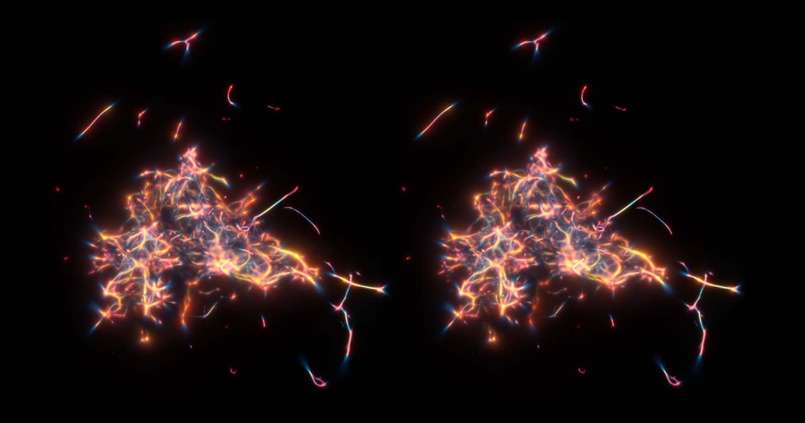
Monte Carlo Physarum Machine:
Characteristics of Pattern
Formation in Continuous
Stochastic Transport Networks
Oskar Elek
University of California, Santa Cruz
Computational Media
Creative Coding Lab
oelek@ucsc.edu
Joseph N. Burchett
New Mexico State University
Department of Astronomy
jnb@nmsu.edu
Abstract We present Monte Carlo Physarum Machine (MCPM):
a computational model suitable for reconstructing continuous
transport networks from sparse 2D and 3D data. MCPM is a
probabilistic generalization of Jones’s (2010) agent-based model for
simulating the growth of Physarum polycephalum (slime mold). We
compare MCPM to Jones’s work on theoretical grounds, and
describe a task-specific variant designed for reconstructing the
large-scale distribution of gas and dark matter in the Universe
known as the cosmic web. To analyze the new model, we first explore
MCPM’s self-patterning behavior, showing a wide range of
continuous network-like morphologies—called polyphorms—that the
model produces from geometrically intuitive parameters. Applying
MCPM to both simulated and observational cosmological data
sets, we then evaluate its ability to produce consistent 3D density
maps of the cosmic web. Finally, we examine other possible tasks
where MCPM could be useful, along with several examples of fitting
to domain-specific data as proofs of concept.
J. Xavier Prochaska
University of California, Santa Cruz
Astronomy and Astrophysics
The University of Tokyo
Kavli Institute for the Physics and
Mathematics of the Universe
jxp@ucsc.edu
Angus G. Forbes
University of California, Santa Cruz
Computational Media
Creative Coding Lab
angus@ucsc.edu
Keywords
Physarum simulation, Monte Carlo,
nature-inspired algorithms, agent-based
modeling, procedural generation
1 Introduction
To understand a process, one must become it: The intelligence that evolved in nature therefore
adapted itself to design pressures presented by various natural processes. To take an example that
is central to this article, the protist Physarum polycephalum (slime mold) has been successfully used
as an unconventional analog computer (Adamatzky, 2010, 2016). As a “thinking machine” and a
creative pattern finder (Adamatzky et al., 2013), Physarum can solve hard spatial problems via its
physical growth—most prominently, finding optimal paths and transport networks connecting sets
of data points where an underlying network structure is expected. The disadvantages, however, are
significant: slow growth of the actual organism, difficulty of feeding it large inputs (e.g., more than
a few dozen data points), and limited dimensionality. For these reasons, it is useful to instead use
a virtual, simulated counterpart—even if not as complex as its biological template—as for many
problems a simulation that qualitatively resembles Physarum’s spatial behavior can be expressive
enough (Jones, 2010, 2015b).
© 2021 Massachusetts Institute of Technology
Published under a Creative Commons Attribution
4.0 International (CC BY 4.0) license.
Artificial Life 28: 22–57 (2021) https://doi.org/10.1162/artl_a_00351
l
D
o
w
n
o
a
d
e
d
f
r
o
m
h
t
t
p
:
/
/
d
i
r
e
c
t
.
m
i
t
.
e
d
u
a
r
t
l
/
/
l
a
r
t
i
c
e
–
p
d
f
/
/
/
/
2
8
1
2
2
2
0
2
8
9
3
2
a
r
t
l
/
_
a
_
0
0
3
5
1
p
d
.
f
b
y
g
u
e
s
t
t
o
n
0
8
S
e
p
e
m
b
e
r
2
0
2
3
O. Elek et al.
Monte Carlo Physarum Machine
Figure 1. Two examples of self-patterning results produced by the presented Monte Carlo Physarum Machine (MCPM)
model. The grayscale insets show similar morphologies in 2D resulting from Jones’s (2010) model, which MCPM
generalizes to 3D by introducing a stochastic behavioral schema for the model agents. (The grayscale insets are from
Jones, 2010.)
The universe of problems involving interconnected network-like structures ever expands in the
Information Age—mostly due to communication and transportation networks (including road and
utility networks, printed circuits, socioeconomic networks, and the Internet). The importance of
epidemiological network modeling has never been as apparent as in 2020/2021. And, in parallel
to humanmade networks, we continue to discover new natural phenomena with significant inter-
connected patterns: from molecular structures, through neuronal networks, circulatory/capillary
systems, fungal and rhizomatic networks, all the way up to the network of dark matter filaments
and intergalactic gas known as the cosmic web. All these phenomena share an important feature: In
one way or another they are built on the notion of optimal transport. Our initial concern in this line
of work has been with the last case: reconstructing the filamentary structures of the cosmic matter
distribution in a consistent and verifiable way.
To this end, we present Monte Carlo Physarum Machine (MCPM): a simulated Physarum machine
that algorithmically mimics the organism’s growth. Relying on Physarum’s ability to closely approx-
imate optimal transport networks, we feed to its virtual counterpart sparse point data as 3D at-
tractors. MCPM’s agents navigate these data to find the most probable paths between them; the
superimposed aggregate of their trajectories then forms the candidate network structure. We cap-
ture the totality of these trajectories as a density field in 3D space, giving rise to continuous network
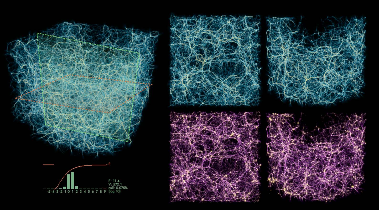
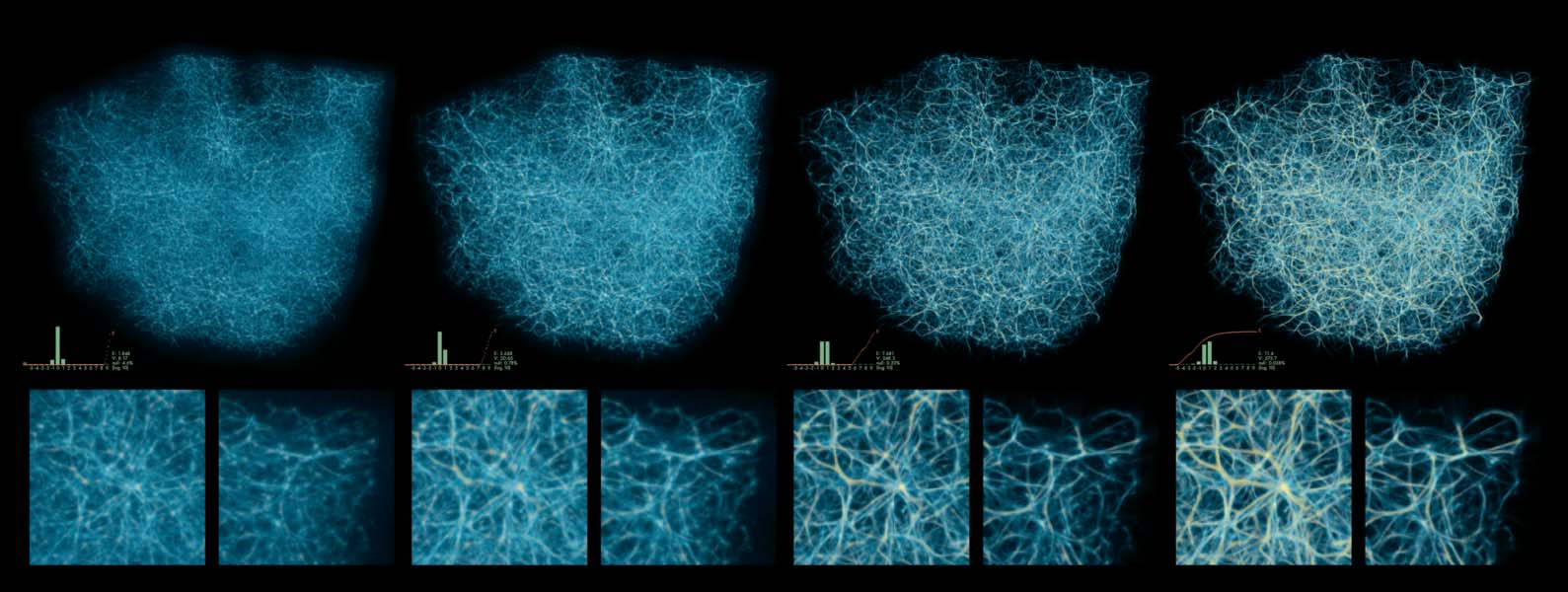
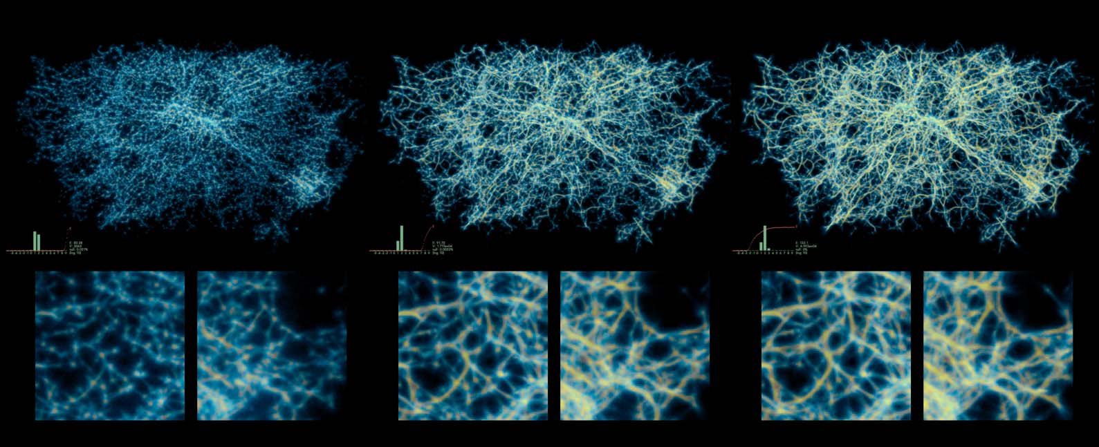
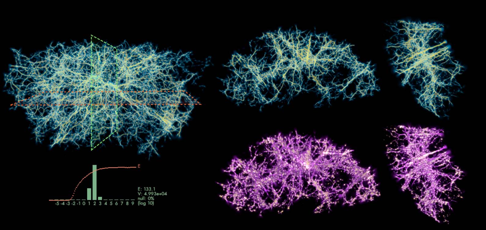
structures which we will refer to as polyphorms. To demonstrate the practicality of the model, we ap-
ply MCPM to galaxy and dark matter halo data sets, interpreting the resulting continuous networks
as proxies for the knots and filaments of the cosmic web.
The first contribution of this article is the full description of the MCPM model (section 4).
MCPM is a generalization of the seminal method described by Jones (2010), from which we draw
much inspiration (section 5; Figure 1). We expand Jones’s work in several ways:
• All decisions in MCPM are stochastic. This makes the model significantly more
customizable, as prior domain-specific knowledge can be encoded in probability density
functions sampled by the model’s agents.
• We extend Jones’s model from 2D to 3D, building on the stochastic formulation. We
achieve this by redesigning the sampling stencil to work with only a binary sensing decision,
rather than performing dense directional sampling as in Jones’s proposed 3D extension
(Jones, 2015b). Consequently, this choice also opens up the future possibility for
higher-dimensional application of the method.
Artificial Life Volume 28, Number 1
23
l
D
o
w
n
o
a
d
e
d
f
r
o
m
h
t
t
p
:
/
/
d
i
r
e
c
t
.
m
i
t
.
e
d
u
a
r
t
l
/
/
l
a
r
t
i
c
e
–
p
d
f
/
/
/
/
2
8
1
2
2
2
0
2
8
9
3
2
a
r
t
l
/
_
a
_
0
0
3
5
1
p
d
.
f
b
y
g
u
e
s
t
t
o
n
0
8
S
e
p
e
m
b
e
r
2
0
2
3
O. Elek et al.
Monte Carlo Physarum Machine
• We add a new data modality decoupled from the algorithm’s signaling mechanism, to
reconstruct the agent distribution. This modality, called a trace, records the collective spatial
history of agents’ positions. After the model reaches equilibrium, the trace provides more
accurate networks in conditions where the agent density by itself would be too low for
getting robust reconstructions.
The second contribution is the case study applying MCPM to data sets whose geometric com-
plexity is higher than that of optimal transport networks but still resembles them to a large degree,
especially with regard to their topology. Here we study the fitting process and reconstruction results
using a task-specific variant of MCPM (section 6), which we have previously applied in the context
of cosmological modeling and visualization (Burchett et al., 2020; Elek et al., 2021; Simha et al.,
2020). We demonstrate how the probabilistic form of MCPM benefits the task of reconstructing
the cosmic web, the structural features of which are best described by a density field, rather than a
network in the strict sense (section 7). We posit that many real-world data sets share this property
and offer several trials to support this (section 8).
2 Background
2.1 Physarum Machines: Real and Virtual
Nature offers a wealth of inspirations for solving difficult computational problems, often referred to
as metaheuristics. Natural selection itself can be framed as a constrained optimization process with
selective pressures acting as design criteria. This is a fact that the tradition of evolutionary compu-
tation builds on (Goldberg, 1989; Hingston et al., 2008), as well as more directly biology-inspired
optimization methods (Mirjalili et al., 2020).
Among the sources of inspirations, one organism clearly shines: Physarum polycephalum, commonly
known as slime mold, has captured the attention of computational researchers over the past two
decades (and half a century longer in biology; Bonner, 2009). The growth patterns of the actual
organism have been used to address many spatial problems: maze solving (Nakagaki et al., 2000),
shortest path finding (Nakagaki et al., 2001), transportation design (Tero et al., 2010), the trav-
eling salesman problem (Jones & Adamatzky, 2014a), and Voronoi diagram estimation (Jones &
Adamatzky, 2015), among others. A survey of this active area of research is given by Sun (2017).
Standing out is the extensive work of Andrew Adamatzky summarized in his books (Adamatzky,
2010, 2016). His team’s recent work goes as far as proposing a Physarum-based hardware for solving
suitable problems (Whiting et al., 2016).
The approach of using Physarum as an analog computer—leading to the moniker Physarum
Machines—has been popular because of the organism’s propensity to systematically explore its en-
vironment for food and shape itself into intricate networks to interconnect with it. Food sources
thus become straightforward proxies for input data, while different chemical and physical stimuli
are available to further steer Physarum’s growth (Adamatzky, 2010).
There are downsides too, however. Physarum grows slowly and is only suitable for small inputs
(approximately up to dozens of distinct points). It is also surface-borne; and while heightfields are
perfectly feasible (Evangelidis et al., 2017), truly 3D volumetric data sets are not. On the other
hand, simulated slime mold—a virtual Physarum machine (VPM)—can be designed to overcome these
obstacles. VPMs usually simulate the organism bottom-up, obtaining Physarum’s approximations from
an iterated composition of simple, local rules.
In this work, we build on the simulation model of Jones (2010). While other computation-
ally efficient VPM models have been proposed—for instance, those based on cellular automata
(Dourvas et al., 2019; Kalogeiton et al., 1986) and formal logic rules (Schumann & Pancerz, 2016)—
we adopt this agent-based model due to its ability to construct precise trajectories. Jones’s model
is related to agent-based modeling of crowds and flocks (Olfati-Saber, 2006; Reynolds, 1987), but
uses a continuous representation of the agents’ density for navigation (Jones, 2010, 2015b). On top
24
Artificial Life Volume 28, Number 1
l
D
o
w
n
o
a
d
e
d
f
r
o
m
h
t
t
p
:
/
/
d
i
r
e
c
t
.
m
i
t
.
e
d
u
a
r
t
l
/
/
l
a
r
t
i
c
e
–
p
d
f
/
/
/
/
2
8
1
2
2
2
0
2
8
9
3
2
a
r
t
l
/
_
a
_
0
0
3
5
1
p
d
.
f
b
y
g
u
e
s
t
t
o
n
0
8
S
e
p
e
m
b
e
r
2
0
2
3
O. Elek et al.
Monte Carlo Physarum Machine
of the successful application to classic problems such as road network optimization (Adamatzky
et al., 2017), this model is suitable for abstract and interactive tasks: B-spline fitting (Jones &
Adamatzky, 2014b), convex and concave hull approximation, and robot navigation (Jones, 2015a).
In our case, it is the model’s ability to approximate optimal transport networks over a set of points that made
it an ideal base for us.
2.2 The Search for the Cosmic Web
The problem that originally motivated this work is the detection and reconstruction of the in-
tergalactic medium (IGM), which forms the large-scale structure of the Universe (also known as
the cosmic web). This section briefly summarizes the existing work in this domain. For more de-
tails, please refer to the comprehensive survey by Libeskind et al. (2018), as well as our prior work
(Burchett et al., 2020; Simha et al., 2020).
Composed mainly of hot gas and plasma, the IGM is purported to trace the underlying dark
matter scaffolding of the cosmic web to contain a significant yet unobserved portion of the Uni-
verse’s conventional matter: at least 40% estimated in total. This refers to the widely known missing
baryon problem (Fukugita et al., 1998). The IGM has long been thought to contain the unaccounted
baryonic matter based on findings from large-scale cosmological simulations, such as the Millenium
(Springel et al., 2005), EAGLE (Schaye et al., 2015), and Bolshoi-Planck (Klypin et al., 2016) simu-
lations. Furthermore, the IGM hydrogen absorption lines frequently detected in spectra of distant
quasars (Lanzetta et al., 1995) have long been assumed to trace the cosmic web structure (Cen
et al., 1994). Recently, astronomers have used the dispersion measure of fast radio bursts to find
the missing baryons, verifying that they reside in the IGM (Macquart et al., 2020); however, im-
portant astrophysical problems remain, as the precise spatial distribution of the IGM is still heavily
underconstrained.
The large-scale simulations also unanimously agree on the expected distribution of the dark
matter and thus the IGM: After billions of years, the combined effect of gravitational attraction
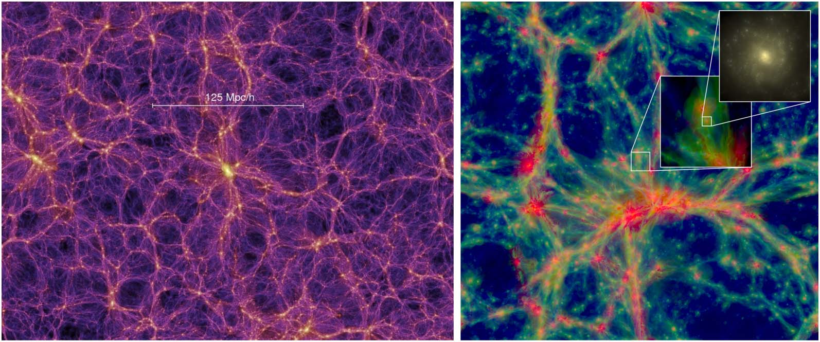
and dark-energetic repulsion has shaped the universe as a vast network (Figure 2). This quasi-fractal
structure (Scrimgeour et al., 2012), widely known as the cosmic web, consists of knots (galaxies
and their clusters) interconnected by a complex network of filaments and separated by vast cells
of significantly under-dense space called voids. In addition, the entire structure is supported by a
scaffolding of dark matter, according to theoretical predictions. These simulations themselves have
been constructed to confirm the earlier findings of the Zeldovich framework (Doroshkevich, 1970;
Icke, 1973; Zeldovich, 1970), which on theoretical grounds predicts the emergence of these very
structures under the influence of the dominant force dynamics known in the Universe.
Figure 2. Illustrating the scale of the cosmic web structures: absolute in megaparsecs (left, Millennium simulation; from
Springel et al., 2005) and relative in comparison to individual galaxies (right, EAGLE simulation; from Schaye et al.,
2015).
Artificial Life Volume 28, Number 1
25
l
D
o
w
n
o
a
d
e
d
f
r
o
m
h
t
t
p
:
/
/
d
i
r
e
c
t
.
m
i
t
.
e
d
u
a
r
t
l
/
/
l
a
r
t
i
c
e
–
p
d
f
/
/
/
/
2
8
1
2
2
2
0
2
8
9
3
2
a
r
t
l
/
_
a
_
0
0
3
5
1
p
d
.
f
b
y
g
u
e
s
t
t
o
n
0
8
S
e
p
e
m
b
e
r
2
0
2
3
O. Elek et al.
Monte Carlo Physarum Machine
The pertinent question is: How do we transfer the indirect knowledge about the cosmic web to actually re-
constructing its structure? By definition, the IGM filaments would consist of diffuse gas that generally
does not emit light at levels detectable by modern telescope instrumentation, making them extremely
challenging to observe directly. On top of that, even the galaxies, which form within filaments and
nodes and serve as the only luminous tracers of the cosmic web, are observable only to a degree. For
instance, with increasing redshift (i.e., distance from Earth), galaxies (particularly fainter ones) are
more difficult to detect and may not be captured by astronomical surveys. We are therefore dealing
with inherently incomplete, heterogeneous data.
The problem can be approached from multiple different angles. The most computationally ame-
nable representations of network structures are based on graphs—the field of combinatorial opti-
mization (Cook et al., 1997; Papadimitriou & Steiglitz, 1998) operates within this paradigm. Graphs
can be regarded as topological structures (Porter & Gleeson, 2016; Woodhouse et al., 2016) or even
as a proxy for 3D geometry (Govyadinov et al., 2019). Similarly, in the astronomical context, both
topological (Aragón-Calvo et al., 2010) and geometric (Chen et al., 2016; Tempel et al., 2014) ap-
proaches use graphs or partially connected graph-like structures as a core representation. Ultimately,
most of the existing approaches have focused on cataloguing and classifying the cosmic large-scale
structure (Libeskind et al., 2018). To our knowledge, no available method is able to recover a com-
plete 3D density map that is inherently driven by the underlying filamentary structure of possibly
incomplete (especially observational) data. Given that the cosmic web is a heterogeneous multi-
scale structure without an intrinsic topology, having an accurate estimate for its density distribution
is bound to benefit many use cases, including our prior work: better understanding the transition
from the galactic to intergalactic environments (Burchett et al., 2020), characterizing the intergalactic
medium toward singular astronomical phenomena (Simha et al., 2020), and potentially shedding new
light on the missing baryon problem itself.
We approached this challenge from the perspective of finding a sound structural interpolator for
the galaxy data, which on the scales where the cosmic web exhibits distinct features (about 1 to 100
Mpc) can be represented as a weighted set of points in 3D space. Optimally, the resulting model has
to enable the following:
• detection of distinct anisotropic structures at least several megaparsecs away from the galaxies,
but ideally providing consistent density estimates in the entire region of interest;
• detection of geometric features across several orders of magnitude in terms of both spatial scale and
density; and
• structural transfer, allowing a calibration of the model on dense simulated data before
deploying it on sparse observed data.
Per our findings, the presented biologically inspired swarm-based approach is able to cover all
the above criteria. In this article, we focus on the simulation and modeling perspective; more details
toward the required astronomical and visualization tasks are provided in Elek et al. (2021).
3 Overview of Methodology
In its core, MCPM is a dynamic computational model defined by a set of priors: a set of probability
density functions and their parameters obtained from domain-specific knowledge and/or fitting to
training data. Once configured, the model can be fitted to input data: a weighted set of points in 2D
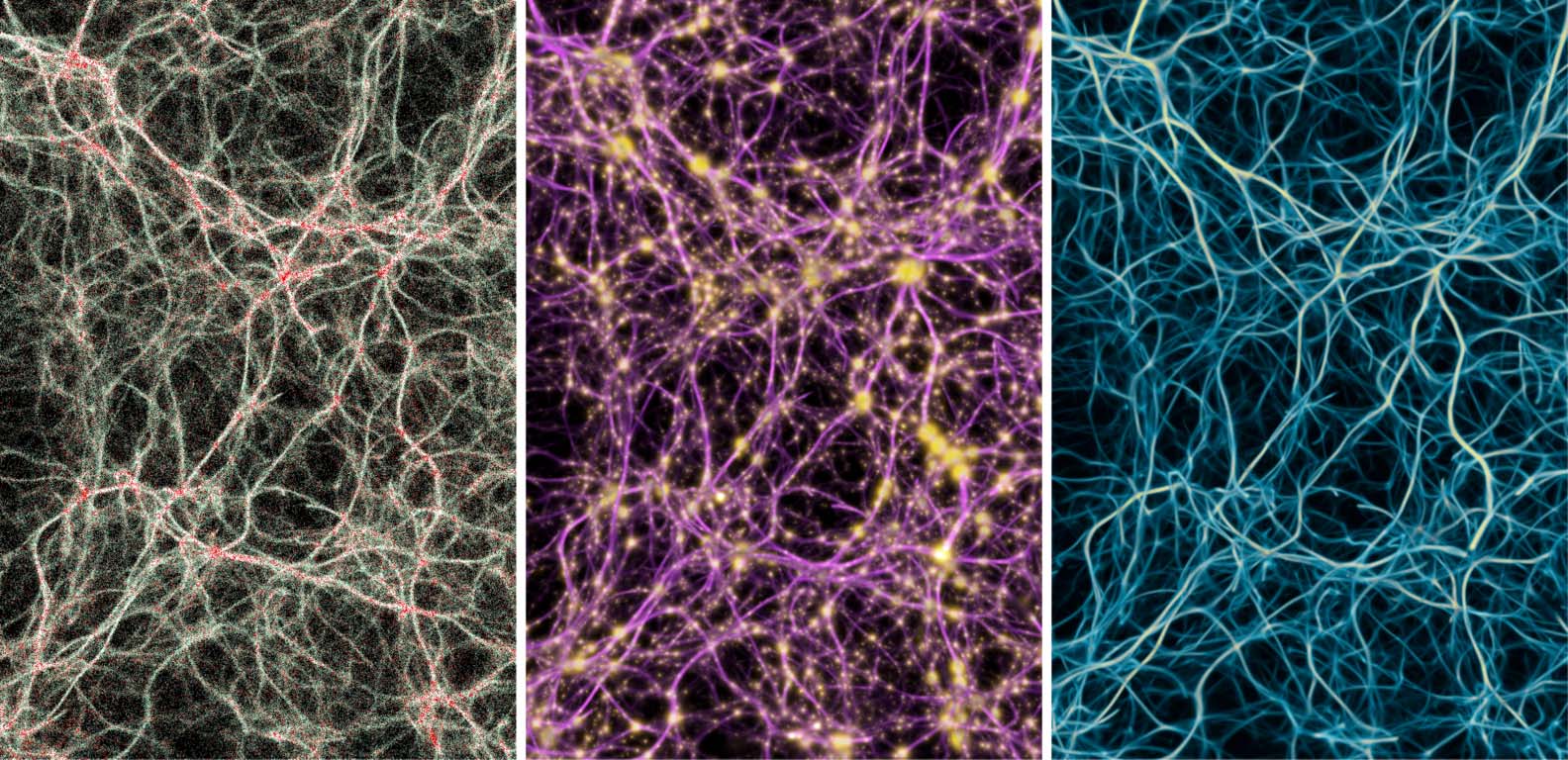
or 3D (Figure 3, left). The result of this fitting is a continuous geometric structure (Figure 3, middle)
which we interpret as a transport network over the input data. Rather than a graph, this geometry is
represented as a density field stored as a densely sampled regular lattice (Figure 3, right).
Section 4 defines the core components of MCPM on an abstract level, i.e., without specifying
the prior probability density functions. In section 5, we outline the differences between MCPM and
the method of Jones (2010) and show that MCPM is the natural generalization of Jones’s method.
26
Artificial Life Volume 28, Number 1
l
D
o
w
n
o
a
d
e
d
f
r
o
m
h
t
t
p
:
/
/
d
i
r
e
c
t
.
m
i
t
.
e
d
u
a
r
t
l
/
/
l
a
r
t
i
c
e
–
p
d
f
/
/
/
/
2
8
1
2
2
2
0
2
8
9
3
2
a
r
t
l
/
_
a
_
0
0
3
5
1
p
d
.
f
b
y
g
u
e
s
t
t
o
n
0
8
S
e
p
e
m
b
e
r
2
0
2
3
O. Elek et al.
Monte Carlo Physarum Machine
Figure 3. Example of a simple continuous transport network reconstructed by MCPM from a set of uniformly dis-
tributed and equally weighted points in 2D. The network is akin to a continuous “fuzzy” triangulation, with MCPM
automatically localizing and connecting to the immediate neighbors of each input point.
Following that, in section 6, we detail the specific version of MCPM that we designed for the task
of finding a meaningful cosmic web map from observational data provided by astronomers: either
galaxies or dark matter halos.
4 Monte Carlo Physarum Machine
Monte Carlo Physarum Machine is a hybrid model—it has a discrete and a continuous component.
The discrete component is an ensemble of particle-like agents that can freely navigate the simulation
domain; these agents serve as a fragmented representation of the virtual organism. The continuous
component is a 3D scalar lattice that represents the concentration of a marker that facilitates informa-
tion exchange between the agents and the data. The model’s behavior is based on a feedback loop
between these two components, executed in two alternating steps: propagation and relaxation (refer
to Algorithms 1 and 2 and the diagrams in Figure 4).
(1) Propagation (Algorithm 1): The propagation step is executed in parallel for each of the agents,
which are the model’s device for exploring the simulation domain. Each agent’s state is represented
by a position and a movement direction, which are stochastically updated (Figure 4(a)–(c)) to navi-
gate through the deposit field (referred to as a “trail” in Jones, 2010; see Figure 4(d); gray cells). The
deposit field is stored as a 3D lattice of scalar values, representing the marker (in biological contexts
usually referred to as chemoattractant) emitted by both the input data points and the agents. The
deposit effectively guides the agents toward the other agents as well as the data: The agents move
with higher likelihood to the regions where deposit values are higher. In addition to the deposit,
we also maintain a scalar trace field (Figure 4(d); green cells), which records the agents’ equilibrium
spatial density but does not participate in guiding them. (A detailed explanation of a trace is provided
in section 5.)
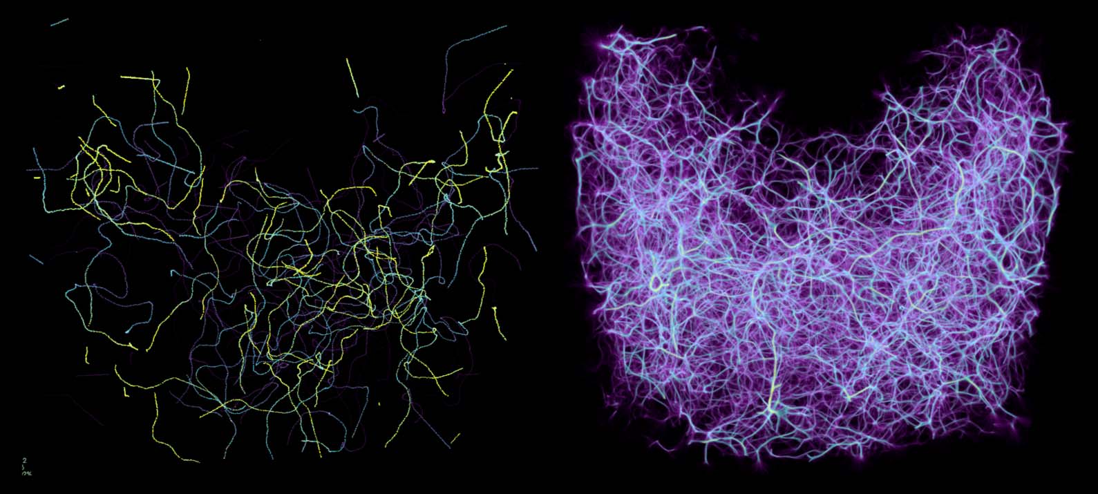
Successive propagation steps build up the agents’ trajectories: random walks that follow the struc-
ture of the deposit field and are recorded in the trace field. While each individual agent draws a
seemingly chaotic path (Figure 5, left), a superposition of many agents averaged over a sufficient
time window results in a smooth converged structure (Figure 5, right).
It is worth noting that the data points are also represented by agents, but of a special type: one
that does not move, but merely emits deposit according to its weight (“mass”). We found this to be
the most consistent way of handling the input data: The relative structural impact of the agents and
the data now simply become a question of tuning the amount of deposit they each emit.
(2) Relaxation (Algorithm 2): The relaxation step ensures that the simulation eventually reaches
an equilibrium. To this end, the deposit field is spatially diffused by a small isotropic kernel and
attenuated—that is, each cell is multiplied by a value <1. The trace field is also attenuated but does
Artificial Life Volume 28, Number 1
27
l
D
o
w
n
o
a
d
e
d
f
r
o
m
h
t
t
p
:
/
/
d
i
r
e
c
t
.
m
i
t
.
e
d
u
a
r
t
l
/
/
l
a
r
t
i
c
e
-
p
d
f
/
/
/
/
2
8
1
2
2
2
0
2
8
9
3
2
a
r
t
l
/
_
a
_
0
0
3
5
1
p
d
.
f
b
y
g
u
e
s
t
t
o
n
0
8
S
e
p
e
m
b
e
r
2
0
2
3
O. Elek et al.
Monte Carlo Physarum Machine
Algorithm 1 Pseudocode for the propagation step.
not diffuse in order to preserve the geometric features in the agents’ distribution, which the
trace represents. (Please refer to section 5 for further discussion on the trace field.)
The simulation reaches its equilibrium when the amount of deposit and trace injected into the
respective fields in the propagation step equals the amount removed by the attenuation in the relax-
ation step. With the parameters used in our experiments (section 7), this usually takes hundreds of
iterations.
4.1 Probabilistic Sampling
The core of MCPM is the agent propagation defined in terms of three probability distributions, the
configuration of which can be tuned in runtime. These are:
• Pdir for sampling the agents’ directional decisions during the sensing and movement phases;
defined on the unit sphere relatively to the current direction of propagation.
• Pdist for sampling the agents’ distance decisions during the sensing and movement phases;
defined in positive real numbers along the current propagating direction.
• Pmut for making the binary mutation decision whether the agent should remain on its
current course or take the newly sampled direction according to Pdir.
By specifying these three distributions, one defines a particular instance of MCPM—we discuss this
further in section 5. For our cosmic web detection task, we detail our choices of these three distri-
butions in section 6.
Now, it is good to take a step back and understand why such a model produces spatial networks
and why these align with the input data. Figure 6 supports this discussion. The key is that the
agents are navigated toward large pools of deposit—this is ensured by defining Pmut such that it
preferentially selects those directions where higher deposit values have been sensed. Agents are
therefore attracted toward data in their vicinity (thus interconnecting them), as well as other nearby
28
Artificial Life Volume 28, Number 1
l
D
o
w
n
o
a
d
e
d
f
r
o
m
h
t
t
p
:
/
/
d
i
r
e
c
t
.
m
i
t
.
e
d
u
a
r
t
l
/
/
l
a
r
t
i
c
e
-
p
d
f
/
/
/
/
2
8
1
2
2
2
0
2
8
9
3
2
a
r
t
l
/
_
a
_
0
0
3
5
1
p
d
.
f
b
y
g
u
e
s
t
t
o
n
0
8
S
e
p
e
m
b
e
r
2
0
2
3
O. Elek et al.
Monte Carlo Physarum Machine
Algorithm 2. Pseudocode for the relaxation step.
Figure 4. Schematic depiction of the agent propagation behavior. By alternating the three stochastic sampling decisions
(a)–(c), every agent describes a random walk (d). By choosing suitable sampling probabilities for the steps (a)–(c), the
agents navigate the structure of the data-emitted deposit field (grey cells) and leave a trace marking their trajectory
(green cells). (Figure image from Elek et al., 2021.)
l
D
o
w
n
o
a
d
e
d
f
r
o
m
h
t
t
p
:
/
/
d
i
r
e
c
t
.
m
i
t
.
e
d
u
a
r
t
l
/
/
l
a
r
t
i
c
e
-
p
d
f
/
/
/
/
2
8
1
2
2
2
0
2
8
9
3
2
a
r
t
l
/
_
a
_
0
0
3
5
1
p
d
.
f
b
y
g
u
e
s
t
t
o
n
0
8
S
e
p
e
m
b
e
r
2
0
2
3
Figure 5. Paths in 3D space drawn by the MCPM agents over 500 propagation steps (section 4). While individual agents
follow a seemingly random set of paths (left), a superposition of the entire swarm reveals an underlying structure
present in the data (right). We store the resulting 3D structure as a density field called a trace.
agents (thus reinforcing existing pathways). The shape characteristics of the network (curvature of
the paths, size, and acuity of the features, as well as connectivity patterns) are further dependent on
the combined influence of Pdir and Pdist. In particular, Pdir needs to be strongly forward-oriented,
which ensures momentum preservation and prevents the agents from getting stuck in local pools of
built-up deposit.
In summary, MCPM solves tasks by acting as a structural interpolator for input data. When
adequately configured and parametrized, it can find natural transport networks that connect neigh-
boring points as a human observer would intuitively do—even in the topologically richer 3D space
Artificial Life Volume 28, Number 1
29
O. Elek et al.
Monte Carlo Physarum Machine
Figure 6. Summary of all the data modalities that MCPM operates with. Left: individual agents (white particles) flowing
among the data points (red particles). Middle: pools of deposit emitted by the data (gold) interconnected by the trace
field (pink). Right: the resulting filamentary structure contained in the trace field, representing the transport network.
(section 7). These networks are represented by the converged trace, i.e., by a continuous density
field rather than an explicit graph.
5 Relation to Max-PM
Our main motivation for extending Jones’s (2010) Max-PM model was the question of parametriza-
tion. While Max-PM is configurable enough to reproduce the morphology of Physarum Polycephalum
and beyond, the agents always respond to different deposit concentrations in the same way: follow
the direction of maximum deposit concentration. Hence the alias Max-PM (with PM standing for Physarum
machine).
At any rate, this behavior—especially after our initial experiments in 3D—led to overly con-
densed pathways and only moderately connected networks (more in section 7; see Figure 7). While
captivating and resembling a 3D Physarum, the fits that Max-PM produced did not match our target
cosmological data well. Another observation was the necessary increase of sampling effort: Max-PM
in 2D uses 1+2 samples for directional sensing; our extension to 3D needs at minimum 1+8 direc-
tions (determined empirically). This increases the sampling effort considerably as well as the number
of access operations to the deposit lattice.
These considerations led us to target the agents’ directional sampling, specifically modifying it
to use stochastic Monte Carlo sampling. In the remainder of this section, we discuss our specific
extensions of Max-PM in detail.
5.1 Stochastic Sampling of Agent Trajectories
The way in which Max-PM treats agent navigation is suitable for the original context: the Physarum
agents use chemotaxis to move around, following the chemoattractant concentration gradient (rep-
resented by the deposit field). In our and arguably many other scenarios—where the main concern
is recovering a network structure that fits target data—we need a more complex behavior that can
be configured based on available knowledge about the data distribution. The main concern is that
in any given geometric configuration of point data, a multitude of feasible pathways is available to
meaningfully interconnect them.
30
Artificial Life Volume 28, Number 1
l
D
o
w
n
o
a
d
e
d
f
r
o
m
h
t
t
p
:
/
/
d
i
r
e
c
t
.
m
i
t
.
e
d
u
a
r
t
l
/
/
l
a
r
t
i
c
e
-
p
d
f
/
/
/
/
2
8
1
2
2
2
0
2
8
9
3
2
a
r
t
l
/
_
a
_
0
0
3
5
1
p
d
.
f
b
y
g
u
e
s
t
t
o
n
0
8
S
e
p
e
m
b
e
r
2
0
2
3
O. Elek et al.
Monte Carlo Physarum Machine
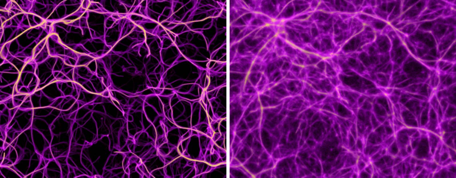
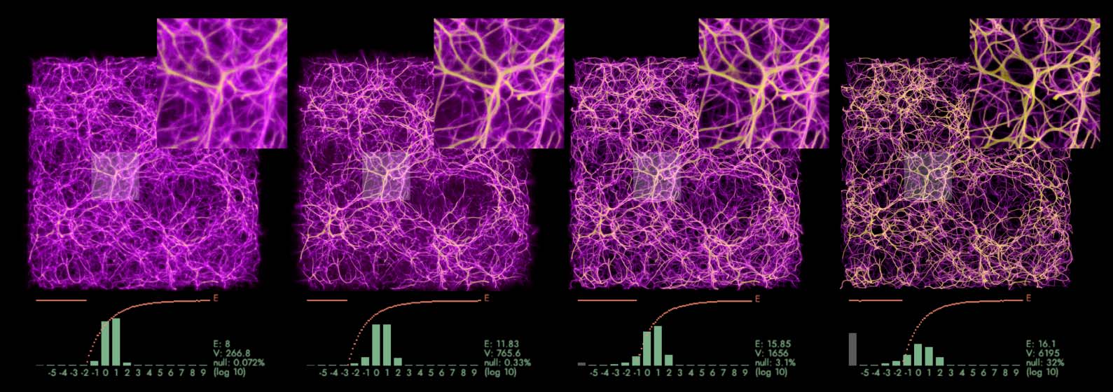
Figure 7. A small segment of a transport network grown on the same data using Max-PM (left) and MCPM (right).
Max-PM yields a clean, well-defined structure, which however does not consistently cover all the input data, in contrast
to the MCPM variant (32% data points missed by Max-PM, compared to 0.072% missed by MCPM).
l
D
o
w
n
o
a
d
e
d
f
r
o
m
h
t
t
p
:
/
/
d
i
r
e
c
t
.
m
i
t
.
e
d
u
a
r
t
l
/
/
l
a
r
t
i
c
e
-
p
d
f
/
/
/
/
2
8
1
2
2
2
0
2
8
9
3
2
a
r
t
l
/
_
a
_
0
0
3
5
1
p
d
.
f
b
y
g
u
e
s
t
t
o
n
0
8
S
e
p
e
m
b
e
r
2
0
2
3
Figure 8. Simple configuration where the agents arriving from data point A need to split evenly between points B and
C (a). In an actual reconstruction scenario, this corresponds to a bundle of agents splitting about evenly and branching
out into two separate filaments (b) and (c), which afterward merge with the flow of the other adjacent agents.
As an example, consider the elementary configuration in Figure 8(a): We want the resulting
network to branch out when connecting the data point A with B and C, which means that the
agent traveling from A has to choose steering toward B or C with roughly the same probability.
This ensures that the aggregate distribution of all agents passing through this location is going to
have a branched shape. In Figure 8(b)–(c) we see an actual such configuration: agents arriving from
the bottom-left branch split into two streams and fluently transition to the more complex region in
the right.
This behavior is represented by the mutation decision (section 4) encoded by the discrete prob-
ability Pmut—that is, whether the agent should remain on its current course, or branch out in the
direction generated in the sensing step.
To provide additional flexibility in representing paths with different scales and curvatures, we
modified the agents’ spatial decisions to behave probabilistically as well, rather than using constant
steps and angles for the agents’ movement (Jones, 2010). This behavior is defined by the continuous
probability density functions Pdir (2D distribution on a sphere) and Pdist (1D distribution on a
half-line).
We can now demonstrate how Max-PM can be framed as a special case of MCPM.
Artificial Life Volume 28, Number 1
31
O. Elek et al.
Monte Carlo Physarum Machine
• Define the mutation probability Pmut as d
∞
1 / (d
ahead of the agent and d1 is the deposit in the mutated direction. Such definition effectively
means that the larger of the deposits will always be selected for the agent to follow.
∞
1 ), where d0 is the deposit value
∞
0 + d
• Define Pdir and Pdist using Dirac delta distributions with the angular and distance
parameters as offsets for the peaks.
In section 6 we discuss the Pdir, Pdist, and Pmut that define the particular variant of MCPM we
employed for reconstructing the cosmic web structure.
5.2 Extension from 2D to 3D
Enabled by the notion of the mutation probability Pmut we can now simplify the sampling stencil—that
is, how many directions need to be sampled during an agent’s sensing stage. We observed that in
Max-PM the network complexity (connectivity) depends on the number of directional samples, and
that this becomes even more pronounced in the topologically richer 3D space.
Given that the directional navigation in MCPM is controlled by Pdir and Pmut, we can reduce
the necessary number of samples to two: one in the forward direction, and one in the mutation
direction. Any direction where Pdir is nonzero can potentially be sampled, and even directions with
low deposit have a chance to be selected (subject to the specific definition of Pmut). This has two
advantages: the savings in directional sampling can be reinvested in increasing the resolution of
the agent’s trajectory, and extensions to higher than three dimensions are now possible without
increasing the sampling effort.
The fact that high-dimensional sampling and integration problems can be effectively solved with
binary sampling stencils is well established in the Monte Carlo community. Both direct (Kajiya, 1986;
Kalos & Whitlock, 2008; Veach, 1997) and Markov-chain Monte Carlo (Hastings, 1970; Metropolis
et al., 1953; Veach & Guibas, 1997) avoid the curse of dimensionality this way when constructing
random walks. Moreover, this strategy can even be the most efficient one, as documented, for
instance, by the ubiquity of path tracing methods for simulating light transport in the visual effects
industry (Christensen & Jarosz, 2016; Fong et al., 2017). Indeed, our method draws significant
inspiration from these works.
5.3 Aggregation of Agent Trajectories
Finally—in addition to the deposit field—we define an additional data modality in MCPM: the trace
field, or simply the trace. Just like the deposit, the trace is stored in a 3D lattice with the same reso-
lution (Figure 4(d) and Figure 6, middle). The trace is computed as a superposition of all locations
visited by each agent within a certain time window—it is an equilibrium spatial distribution of agent
trajectories. Please refer to the pseudocode in Algorithms 1 and 2 for how the trace is constructed
on the algorithmic level—formally, we can define it as a probability density PT over positions x in
3D space:
PT(x) = n · E[ N(x)]
where N is the number of agents in the cell adjacent to x, and n is a normalization constant. The
expected value of N(x) is the Monte Carlo estimate calculated as a moving average, as a function of
the attenuation parameter (cf. the pseudocode for the relaxation step in Algorithm 2).
Rather than using the deposit to recover the reconstructed network (as in Jones’s method (2010,
2015b)) we use the trace for this purpose. This has multiple advantages:
(1) Resolution: In contrast to the deposit, the trace field is not subject to spatial
diffusion—structural details are therefore preserved (Figure 9).
32
Artificial Life Volume 28, Number 1
l
D
o
w
n
o
a
d
e
d
f
r
o
m
h
t
t
p
:
/
/
d
i
r
e
c
t
.
m
i
t
.
e
d
u
a
r
t
l
/
/
l
a
r
t
i
c
e
-
p
d
f
/
/
/
/
2
8
1
2
2
2
0
2
8
9
3
2
a
r
t
l
/
_
a
_
0
0
3
5
1
p
d
.
f
b
y
g
u
e
s
t
t
o
n
0
8
S
e
p
e
m
b
e
r
2
0
2
3
O. Elek et al.
Monte Carlo Physarum Machine
(2) Specificity: Recovering the network from the trace becomes much easier than from the
deposit, as in the latter, the data term has by design a much higher impact than the agent
term.
(3) Interpretability: While the exact mathematical properties of the trace in relation to Pmut,
Pdir, and Pdist are as yet unknown, they are nevertheless in a direct relationship. One way to
interpret the trace is the total probability of the agents’ distribution marginalized over all
possible geometric configurations that can occur in a given data set.
Another way of interpreting the trace is that it provides a continuous estimate of the geometric
and topological structure outlined by the input data. This is related to the use of such a structure
by Jones and Saeed (2007), referred to as a trail in their work. The application of a trail here was
to substitute for standard image-processing kernels, as used for denoising or contrast enhancement.
Unlike their trail, the trace lives in a different frame of reference than the input data: The data are
sparse and unordered points, while the trace is a function densely sampled in space and continuous.
Other than that, these data structures are conceptually similar.
To succinctly describe the trace in text, we use term polyphorm to refer to the particular continuous
geometries represented by the trace field, as well as a general label of the concept of a continuous
transport network, i.e., a network implicitly defined by the trace density field (as opposed to a
network explicitly represented by a graph or other means).
5.4 Fully Continuous Representation
Our last design choice is to fully decouple the representation of agents and the underlying discrete
data structures. In Max-PM, only one agent can be present in each cell of the deposit field at any
given time. This is suitable for simulating the actual organism, as each agent represents a small
fragment of the body and therefore occupies a certain volume of space.
In our case, this behavior is no longer desired: Our agents represent an abstract spatial distribu-
tion with possibly several orders of magnitude in dynamic range. For instance, cosmic overdensities
−3 and 102 are important in the astrophysical inquiry. We therefore allow agents to move
between 10
freely without enforcing any limit on their number in each grid cell. This has additional benefits: It
decreases the amount of necessary bookkeeping, and decouples the reconstructed network structure
from the data structures’ resolution (as demonstrated in section 7).
6 MCPM for Cosmic Web Mapping
In sections 4 and 5 we described the components of MCPM and provided the rationale behind our
design. Now we specify the probabilities Pdir, Pdist, and Pmut, which together define the variant of
MCPM used in our previous work (Burchett et al., 2020; Elek et al., 2021; Simha et al., 2020) for
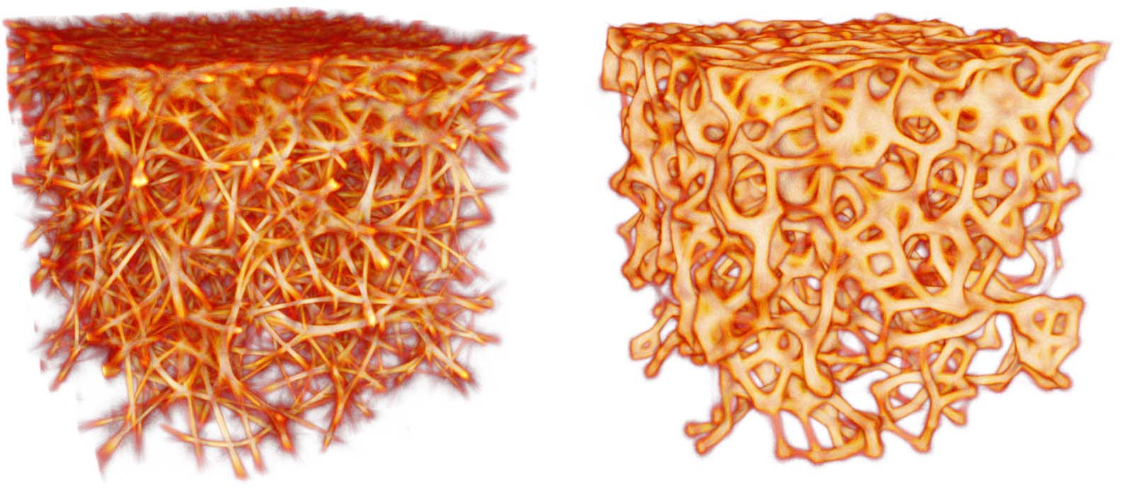
Figure 9. Comparison of the distribution of data-emitted deposit (gold) and the reconstructed trace field (purple) in
two sample configurations. While the deposit field is sparse and diffused, the trace is continuous and sharp, and thus
serves as a better estimate of the transport network.
Artificial Life Volume 28, Number 1
33
l
D
o
w
n
o
a
d
e
d
f
r
o
m
h
t
t
p
:
/
/
d
i
r
e
c
t
.
m
i
t
.
e
d
u
a
r
t
l
/
/
l
a
r
t
i
c
e
-
p
d
f
/
/
/
/
2
8
1
2
2
2
0
2
8
9
3
2
a
r
t
l
/
_
a
_
0
0
3
5
1
p
d
.
f
b
y
g
u
e
s
t
t
o
n
0
8
S
e
p
e
m
b
e
r
2
0
2
3
O. Elek et al.
Monte Carlo Physarum Machine
the cosmic web reconstruction task. We likewise use it in the experiments throughout section 7 and
most of the article.
Directional distribution Pdir
The main criterion for Pdir is that the agents should maintain a certain momentum—otherwise, if
allowed to turn too rapidly, they would invariably get stuck in the local maxima of the deposit field.
The simplest choice here is uniform distribution over the forward-facing cone of directions. This
distribution is parametrized by a single scalar parameter: the opening angle of the cone. Routines
for efficiently drawing samples from this distribution can be found, for instance, in Watson (1982).
Other viable choices of Pdir include the spherical Gaussian, the von Mises–Fisher distribution
(Fisher, 1953), the Henyey–Greenstein distribution (Henyey & Greenstein, 1941), and their trun-
cated versions.
When configuring Pdir, the rule of thumb we used in our fitting confirms the findings of Jones
(2010): The sensing angle should be larger than the mutation (i.e., turning) angle. We typically use
twice the value for sensing than for turning. The variation of these and other parameters is further
explored in section 7.
Distance distribution Pdist
Since the cosmic web is built up from filaments consisting mostly of hot gas, we use the
Maxwell–Boltzmann distribution for sampling the agents’ sensing and movement distances. This
statistical distribution describes the velocity dispersion of particles in idealized gas and plasma
(Mandl, 1988), which makes it suitable for our use case and potentially for modeling other physical
systems. Efficient sampling from this distribution is described, for example, by Hernandez (2017).
Other good candidates for Pdist include the exponential distribution (e.g., to model bacterial
motion dynamics (Li et al., 2008)), log-normal (for particles under Brownian motion), Poisson,
Gamma, and other distributions defined in R+. Convex combinations of multiple modes are also
possible, if different distinct scales of features are expected in the modeled system. The weight of
the tail in Pdist determines the range of feature scales MCPM will be able to reconstruct: In the
simplest case of constant sensing and movement distances, the model will be sensitive to only one
characteristic feature size.
When generating the sensing and movement distances for an agent, we use the same seed to
sample Pdist—this is to avoid the cases when the movement distance would exceed the sensing
distance. Even more so than in the directional sampling, here we find that the sensing distance
should be significantly larger than the movement distance: A good starting point is a difference of
about an order of magnitude.
Mutation probability Pmut
In contrast to distributions Pdir and Pdist, mutation probability Pmut is a binary probability that an
agent deviates (branches away) from its current course. Its definition needs to ensure that agents
predominantly steer toward a higher concentration of the deposit. (This, in our experience, is the
sufficient condition for the simulation to equilibrate in a configuration that follows the data.) If this
were the opposite case, the agents would actually be repulsed by the data, as well as from each other.
With reference to the pseudocode in Algorithms 1 and 2, we define Pmut as
Pmut(d0, d1, s) = ds
1
/(ds
0
+ ds
1
)
where d0 is the deposit in the forward direction, d1 is the deposit in the mutated direction, and
s >= 0 is the sampling exponent. We examine the impact of the sampling exponent (and other
parameters) on the resulting network geometry in section 7.
An alternative definition of Pbranch could assume that the agents move in a participating medium
with density proportional to the deposit, in which case the agent dynamics would be subject to
34
Artificial Life Volume 28, Number 1
l
D
o
w
n
o
a
d
e
d
f
r
o
m
h
t
t
p
:
/
/
d
i
r
e
c
t
.
m
i
t
.
e
d
u
a
r
t
l
/
/
l
a
r
t
i
c
e
–
p
d
f
/
/
/
/
2
8
1
2
2
2
0
2
8
9
3
2
a
r
t
l
/
_
a
_
0
0
3
5
1
p
d
.
f
b
y
g
u
e
s
t
t
o
n
0
8
S
e
p
e
m
b
e
r
2
0
2
3
O. Elek et al.
Monte Carlo Physarum Machine
the eikonal equation and Pmut could be derived from the Beer–Lambert law. This is not our case,
however, as collisions between the intergalactic medium particles do not have appreciable impact
on the cosmic web geometry.
It is worth noting that by increasing the values of the sampling exponent we approach the limit
case discussed in section 5, i.e., MCPM becomes identical with Max-PM for s → ∞.
7 Experiments
Our open-source implementation of MCPM called Polyphorm (Elek and Forbes, 2021) is written
in C++ and uses DirectX with GPU compute shaders for executing the parallel propagation and
relaxation steps, as well as facilitating an interactive visualization.
Our GPU implementation was developed on an NVIDIA TitanX, and is capable of fitting 10
million agents over 1, 0243 deposit/trace grids at roughly 150–200 ms per model iteration, with
an additional 30–100 ms needed for the visualization. Including the agents and rendering buffers,
no more than 6 GB GPU memory is consumed at that resolution, using float16 precision to store
both the deposit and trace grids. In all our experiments the model converges in fewer than 700
iterations (about 1–3 min of real time). It is thanks to the massive parallelism of modern GPUs,
combined with the high locality of memory accesses in MCPM, that we are able to simulate 10M or
more agents at interactive rates. This is essential for obtaining noise-free simulation results. Further
performance data are available in Elek et al. (2021).
The performance scales close to linear with the number of voxels, and sub-linearly with the
number of agents: 100M agents runs at 300 ms ceteris paribus, that is 10× more agents at only 2×
the slowdown (compared to 10M agents). Using more agents has minimal impact on the model’s
spatial details, but it does increase effective resolution by proportionally reducing the Monte Carlo
noise levels.
All of the model’s parameters (specific values are provided in the following subsections, with
reference to the pseudocode in Algorithms 1 and 2) can be modified at any point during the simu-
lation, which allows for easy tuning of the resulting 3D polyphorm structures. Edits typically take
several seconds to manifest, both visually and in the value of the loss function (in Section 7.3 we
discuss the details of our employed loss function).
We rely on cosmological data sets to conduct the practical part of the evaluation, in which we
focus on fitting the model. These include the Bolshoi-Planck large-scale cosmological simulation
(Klypin et al., 2016) at zero redshift (i.e., corresponding to the present-day Universe) with 840K
dark matter halos extracted by the Rockstar code (Behroozi et al., 2012). These are simulated data
with a priori known ground-truth cosmic web structure, which is why we use that to calibrate
the MCPM parameters. Our target data set for reconstructing the cosmic web structure comprises
37.6K galaxies (their locations and masses) from the Sloan Digital Sky Survey (SDSS) catalog (Alam
et al., 2015), spanning redshifts between 0.0138 and 0.0318. For more details about the astronomical
evaluation of our results, please refer to Burchett et al. (2020) and Simha et al. (2020). Here we will
be concerned with the behavior of MCPM and the geometry generated by it.
For the visualizations, we use direct volume rendering (Beyer et al., 2015) (for field data) and
particle rendering (for the agents). Sometimes, in addition to projections of the full 3D data, we
isolate slices and cross sections where better insight is necessary. Full exposition of our visualization
methodology is provided in Elek et al. (2021).
All the following experiments use the MCPM variant defined in section 6, unless explicitly
mentioned.
7.1 Self-Patterning
Even though we primarily care about the data-driven mode of operation, we start by looking at
polyphorms produced by the model without any prior stimuli. In the following examples we work
with a 5403 simulation grid uniformly filled with 2M agents at the start of the simulation.
Artificial Life Volume 28, Number 1
35
l
D
o
w
n
o
a
d
e
d
f
r
o
m
h
t
t
p
:
/
/
d
i
r
e
c
t
.
m
i
t
.
e
d
u
a
r
t
l
/
/
l
a
r
t
i
c
e
–
p
d
f
/
/
/
/
2
8
1
2
2
2
0
2
8
9
3
2
a
r
t
l
/
_
a
_
0
0
3
5
1
p
d
.
f
b
y
g
u
e
s
t
t
o
n
0
8
S
e
p
e
m
b
e
r
2
0
2
3
O. Elek et al.
Monte Carlo Physarum Machine
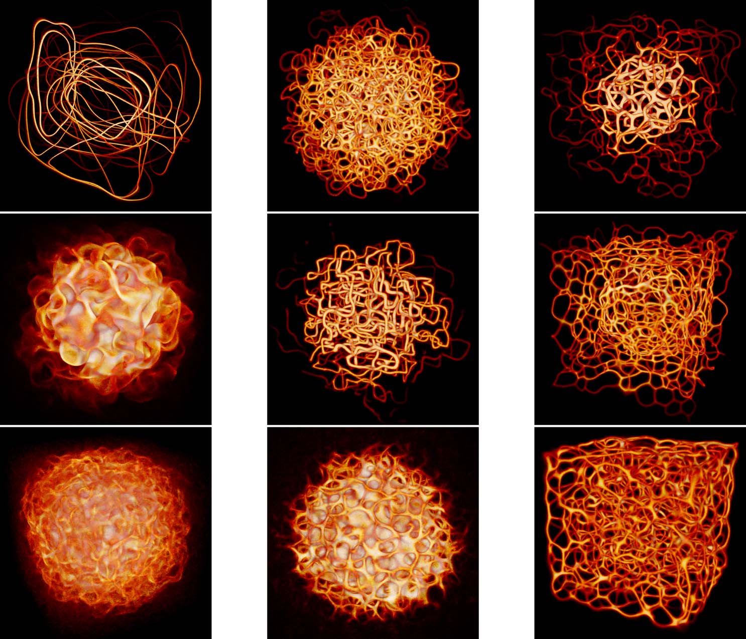
In line with Jones’s (2010) findings we observe that the free patterns created by MCPM are stable
in the qualitative sense. That means that for any given parametrization the generated features will be
comparable, but rarely static: The generated polyphorms are in constant flux. In the experiment in
Figure 10 we explore a number of configurations that led to distinctive results. This experiment was
conducted in a single session, changing one or multiple MCPM parameters at a time and waiting for
the simulation to sufficiently converge after resetting the agents to random initial positions.
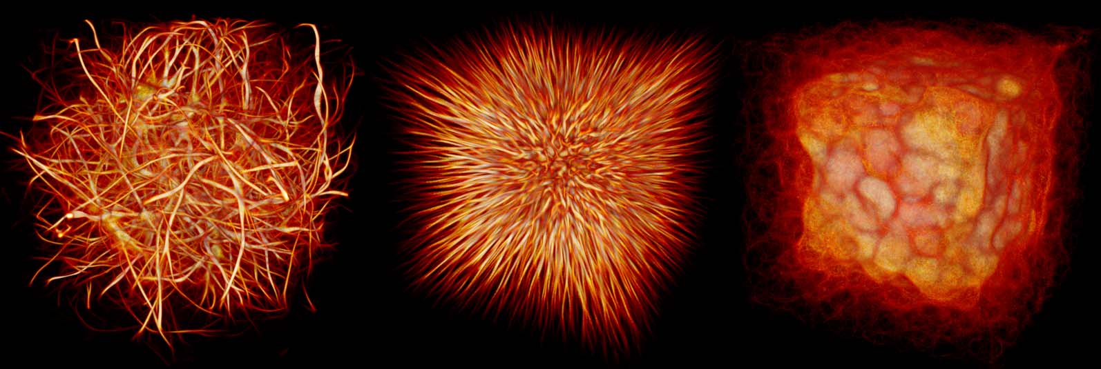
In addition to these meta-stable patterns, a plethora of transient ones is accessible. These occur
when the model’s configuration changes significantly, as a sort of dynamic phase change. Figure 11
shows a few illustrative examples of serendipitous trips through the parameter space. Given that
these forms are dependent on the momentary state of the model before the phase change, and are
unique to both the original and modified parametrization, there is currently no way to enumerate
them systematically.
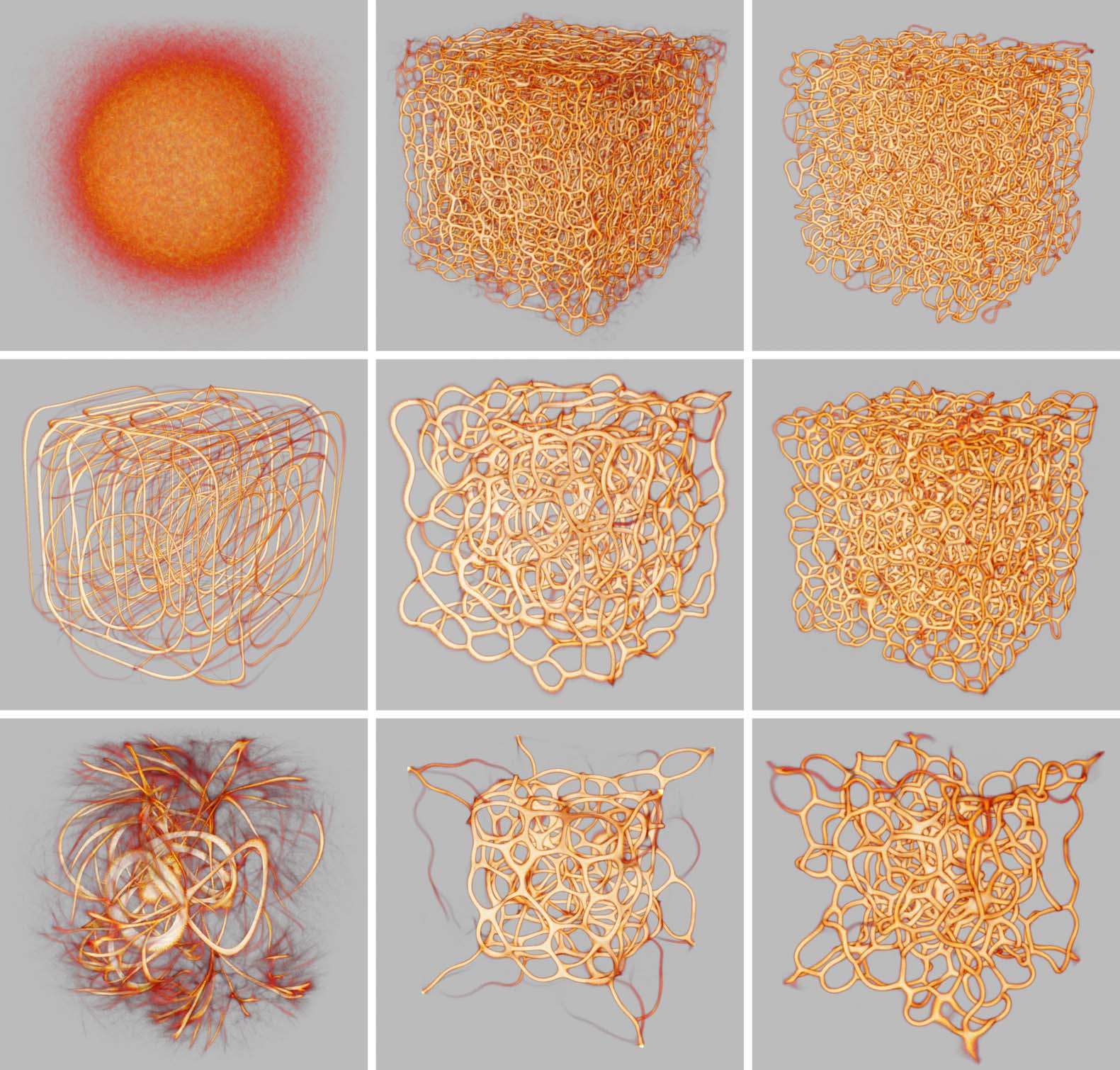
Even though all the parameters impact the polyphorm, the most significant determinants
of shape are the sensing angle, the sensing distance, and the respective movement parameters.
These were the parameters we adjusted the most frequently during fitting. In the experiment
illustrated in Figure 12 we therefore focused on exploring these fitting dimensions. Curiously, we
l
D
o
w
n
o
a
d
e
d
f
r
o
m
h
t
t
p
:
/
/
d
i
r
e
c
t
.
m
i
t
.
e
d
u
a
r
t
l
/
/
l
a
r
t
i
c
e
–
p
d
f
/
/
/
/
2
8
1
2
2
2
0
2
8
9
3
2
a
r
t
l
/
_
a
_
0
0
3
5
1
p
d
.
f
b
y
g
u
e
s
t
t
o
n
0
8
S
e
p
e
m
b
e
r
2
0
2
3
Figure 10. Interesting polyphorms the model generates without any pre-patterning cues, including features like tubular
filaments, loops, fuzzy membranes, thin fibers, branches, and undulating pulses. Some of these morphologies closely
resemble those in Jones (2010), such as (d), (f), and (h); others are similar but topologically connected in novel ways,
e.g., (i), and others still are completely novel, e.g., (a), (b), and (c). In all of these results, a weak attracting force toward
the center of the domain has been applied to the agents in order to prevent crowding along the edges, which can
sometimes happen. Starting at (a), every subsequent change of MCPM parameters is highlighted. The parameters (see
pseudocode in section 4) are sensing angle (SA), sensing distance (SD), move angle (MA), move distance (MD), sampling
exponent (SE), agent deposit (De), and field persistence (Pe). The size of the simulation domain is 100 units in each
dimension.
36
Artificial Life Volume 28, Number 1
O. Elek et al.
Monte Carlo Physarum Machine
Figure 11. Unstable polyphorms generated by MCPM, representing phase transitions between different configurations.
A focused examination of transient phenomena generated by another Physarum simulation has been done by Jenson
and Kuksenok (2020), studying the interaction with complex artistic and didactic systems.
observed correlation between the stability of the fit and how interconnected the network structure
is: The polyphorms in the upper right part of the figure were much more persistent in time than
those in the left.
Another important design dimension is to consider different behaviors of the agents. In particu-
lar, many natural systems contain repulsion as another important shaping force. Encoding this type
of behavior in MCPM simply means reversing the sampling decision given by Pmut (Algorithms 1
and 2). Consequently, the agents will navigate toward lower deposit concentrations, i.e., locations
not occupied by other agents or data points. More complex repulsion behaviors could also be en-
coded through specialized redesigns of Pdir and Pmut.
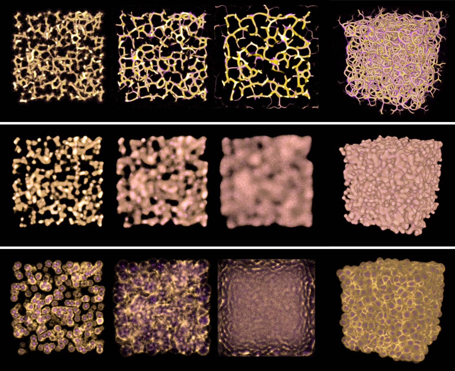
Figure 13 documents three MCPM runs in 1, 0243 simulation grids and 10M agents, comparing
the original attractive agent behavior, its repulsive inversion, and a 50/50 mix of the two behaviors.
In line with the previous experiments, the attractive behavior leads to a network-like polyphorm
that, after forming, remains relatively stable and slowly condenses to a thicker and sparser structure.
On the other hand, the repulsive behavior forms cellular patterns around the sites where they were
initialized. These patterns are only transient, however: As the agents continue repelling each other,
the pattern breaks down and dissipates. Finally, the mixed behavior—where each agent randomly
decides to be attracted or repelled by a deposit—leads to a structure that is a blend of both: sites
form cells, neighboring sites merge together, and the resulting interconnected structure slowly dif-
fuses. Figure 13 maps the temporal progression of each regime, and additionally shows a 3D view
of the entire structure at a point when its features are most visible.
7.2 Uniform Stimuli
We now start introducing data in homogeneous configurations. We show that MCPM produces
meaningful networks over points with different uniform distributions in 3D: in a regular lattice
(Figure 14), distributed randomly (Figure 15), and following a low-discrepancy blue noise distribution
(Ahmed et al., 2016; Figure 16).
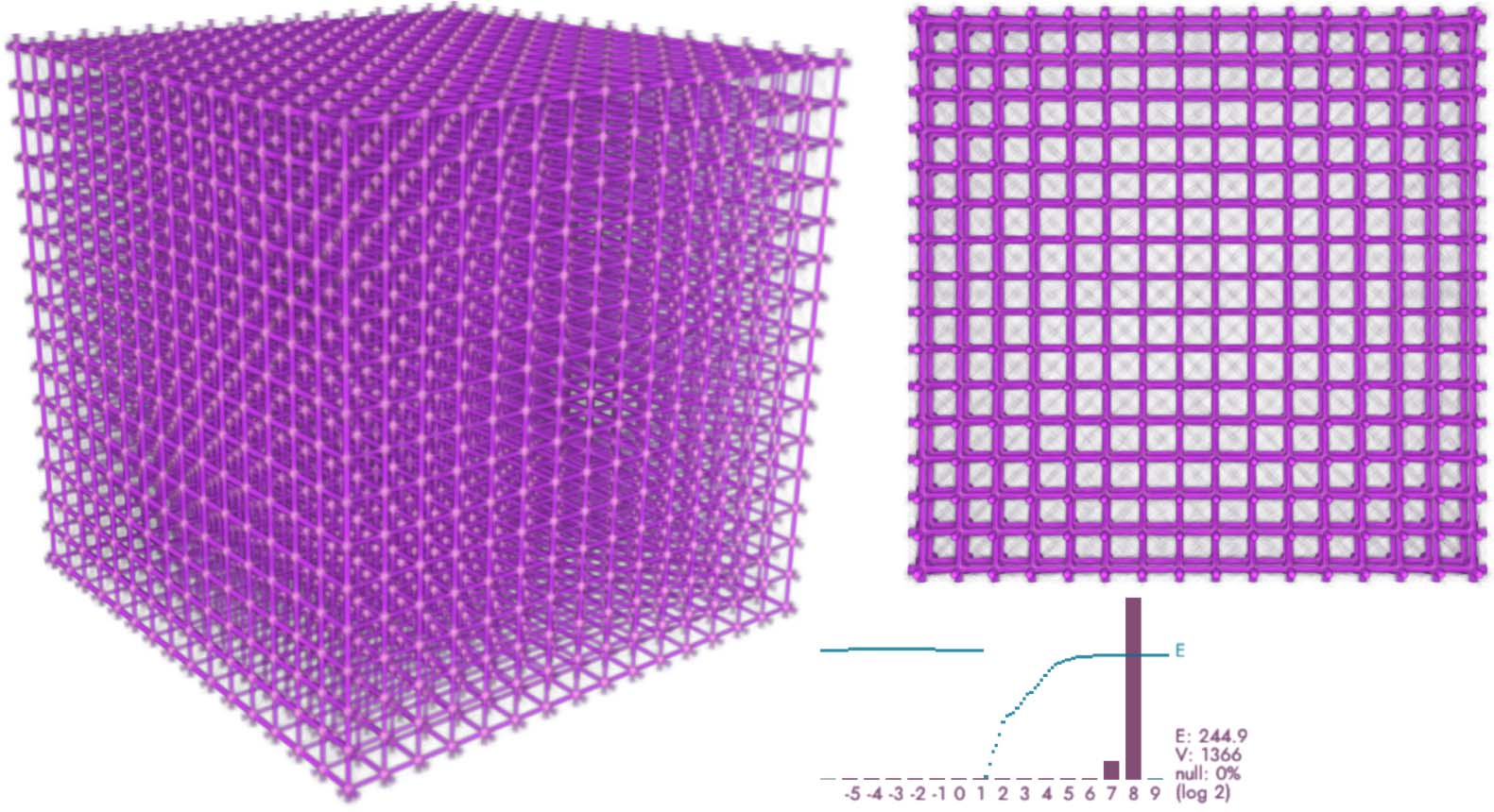
In a regular lattice (Figure 14) MCPM robustly finds straight connections between points and,
due to the multiscale movement of the agents (cf. section 6), also the diagonals of the sub-boxes.
The model can be tweaked to prefer the diagonals simply by increasing SD to about 70–80 vox.
The fitting takes about 300 iterations of the model to converge (see the discontinuity in the
energy plot in Figure 14, bottom, where we restarted the fitting process). Remarkably all the data
points receive nearly identical density of the agents, as shown in the histogram.
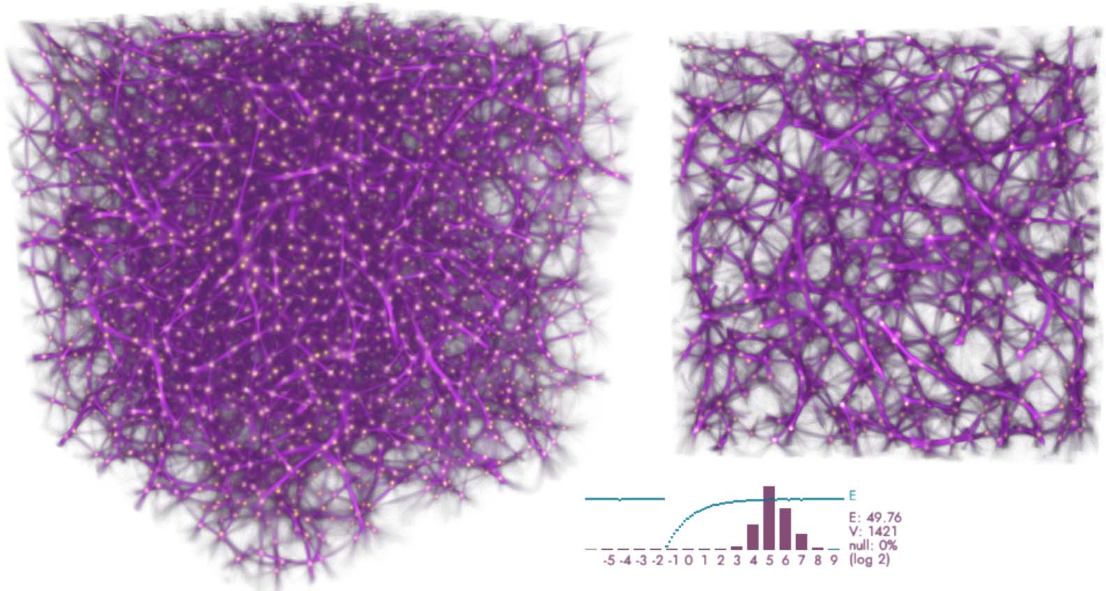
Randomly distributed points (Figure 15) have a tendency to cluster, leading to a spurious rein-
forcement of some of the fitted network connections. As a result, fitting from uniformly initialized
agents takes somewhat longer, about 500 iterations. The density histogram at data points is close to
Gaussian, with a slight positive skew, and variance proportional to the density fluctuation of the data.
Artificial Life Volume 28, Number 1
37
l
D
o
w
n
o
a
d
e
d
f
r
o
m
h
t
t
p
:
/
/
d
i
r
e
c
t
.
m
i
t
.
e
d
u
a
r
t
l
/
/
l
a
r
t
i
c
e
–
p
d
f
/
/
/
/
2
8
1
2
2
2
0
2
8
9
3
2
a
r
t
l
/
_
a
_
0
0
3
5
1
p
d
.
f
b
y
g
u
e
s
t
t
o
n
0
8
S
e
p
e
m
b
e
r
2
0
2
3
O. Elek et al.
Monte Carlo Physarum Machine
l
D
o
w
n
o
a
d
e
d
f
r
o
m
h
t
t
p
:
/
/
d
i
r
e
c
t
.
m
i
t
.
e
d
u
a
r
t
l
/
/
l
a
r
t
i
c
e
–
p
d
f
/
/
/
/
2
8
1
2
2
2
0
2
8
9
3
2
a
r
t
l
/
_
a
_
0
0
3
5
1
p
d
.
f
b
y
g
u
e
s
t
t
o
n
0
8
S
e
p
e
m
b
e
r
2
0
2
3
Figure 12. Varying the sensing angle (SA) horizontally and the sensing distance (SD) vertically. The move angle is fixed
at half the SA and move distance at a constant 0.1, sampling exponent 3.0, agent deposit 2.0, and persistence 0.9. The
domain size is 100 units.
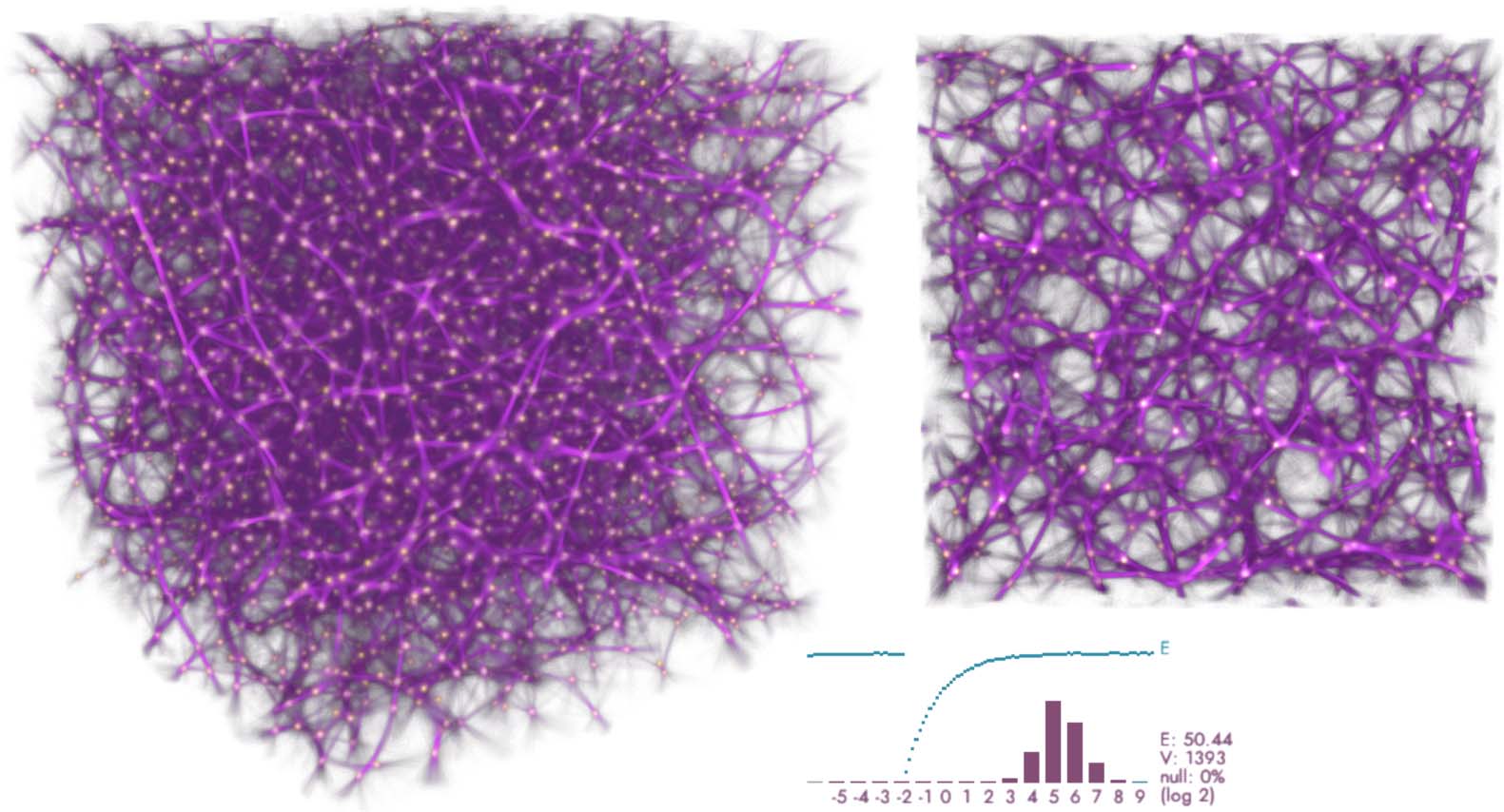
In Figure 16, using a low-discrepancy Poisson-like distribution of the data (Ahmed et al., 2016),
we obtain perhaps the most organic of homogeneous patterns. Since the low-discrepancy points
emulate the distribution of cells in biological tissues (and similar such phenomena), the resulting fit
resembles a natural scaffolding, not unlike bone marrow (also cf. section 8.3). The structure also
bears resemblance to rhizomatic systems (such as tree roots and mycelial networks).
Fitting takes about 500 iterations and results in a density distribution not unlike the random
case, but with a slightly stronger positive skew. Tweaking the values of SE and then trying different
distance sampling distributions would impact the acuity of the fitted network, and would expand or
narrow the resulting distribution histogram.
7.3 Fit Energy (Loss Function)
MCPM solves the problem of reconstructing a volumetric transport network over a set of discrete
points. The network should include all input points, perhaps except for outliers. We also want the
weight of the input points to influence the strength of the network connections, i.e., to attract more
agents.
38
Artificial Life Volume 28, Number 1
O. Elek et al.
Monte Carlo Physarum Machine
l
D
o
w
n
o
a
d
e
d
f
r
o
m
h
t
t
p
:
/
/
d
i
r
e
c
t
.
m
i
t
.
e
d
u
a
r
t
l
/
/
l
a
r
t
i
c
e
–
p
d
f
/
/
/
/
2
8
1
2
2
2
0
2
8
9
3
2
a
r
t
l
/
_
a
_
0
0
3
5
1
p
d
.
f
b
y
g
u
e
s
t
t
o
n
0
8
S
e
p
e
m
b
e
r
2
0
2
3
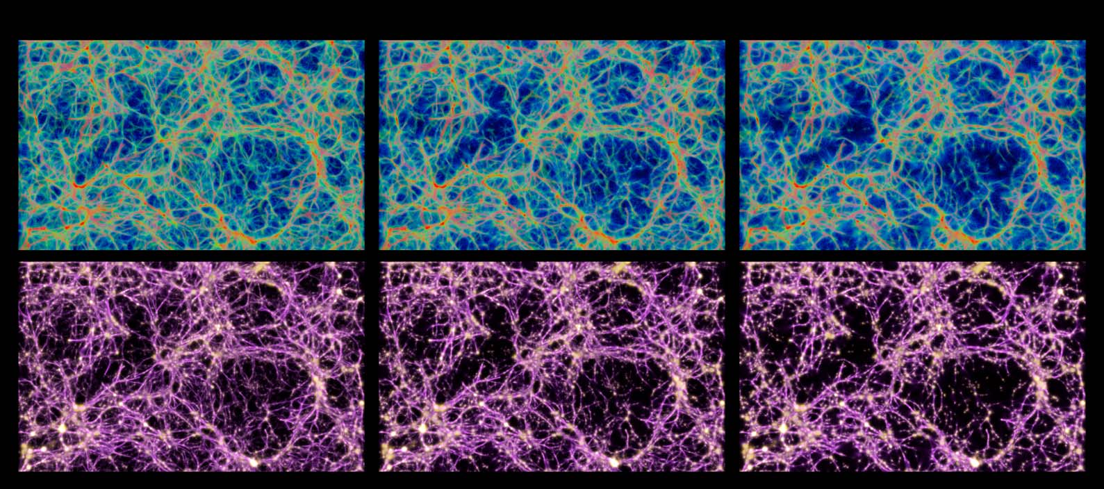
Figure 13. Polyphorms generated by an ensemble of attractive agents (i.e., the base MCPM, top row), repulsive agents
(bottom row), and a 50/50 combination of the two behaviors (middle row). The agents were initialized at random
sites in a domain 100 units in size, with no data present. The visualization shows a superposition of both the trace
(purple) and the deposit (yellow). All the experiments were generated using the following parameters: sensing angle
60 deg, move angle 30 deg, sensing distance 3.0, move distance 0.05, agent deposit 10.0, persistence 0.95, and sampling
exponent 5.0.
The energy function we have used for fitting encapsulates all of the above considerations. To
compute the energy I of the current MCPM fit, we compute the mean of the trace values summed
over the input data point locations, normalized by the data points’ weights:
I(trace) =
1
data.count
(cid:2)
d ∈ data
trace[ d.pos]
d.weight
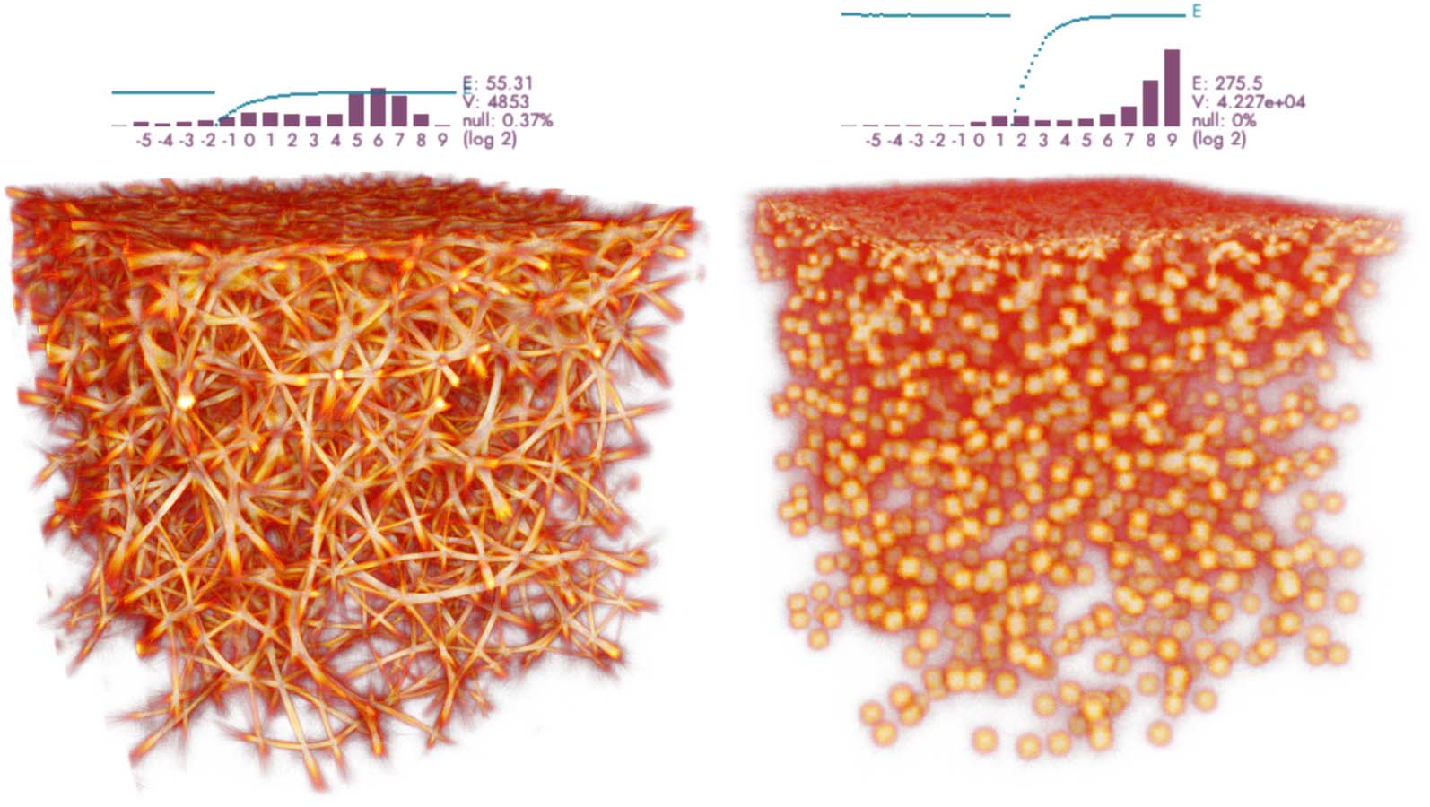
This design has one shortcoming: Collapsed fits can occur, where all the agents are attracted to
the nearest data point (Figure 17, right). Compared to a “healthy” transport network (Figure 17,
left), the collapsed fit lacks connections between neighbors, rather resulting in a disconnected set
of “blobs.” Since there is no established definition of connectedness in this context, we leave this
aspect for visual evaluation and use the above defined energy function only to explore the fitting
parameter space locally. The interactive visualization in Polyphorm and the ability to inspect the fit
by slicing and different rendering modes was therefore essential to obtaining good reconstruction
results (Elek et al., 2021).
Artificial Life Volume 28, Number 1
39
O. Elek et al.
Monte Carlo Physarum Machine
Figure 14. Regular lattice of 163 = 4K points, simulated using deposit/trace grids with 7203 voxels (vox), 10M agents,
sensing distance (SD) 50 vox, move distance (MD) 0.65 vox, sensing angle (SA) 20 deg, move angle (MA) 10 deg, and
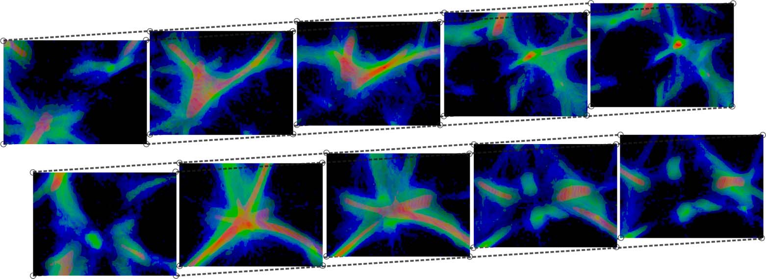
sampling exponent (SE) 5. The plot shows the log-2 histogram of trace readouts at the data points (bordeaux) and the
fit energy (cyan).
l
D
o
w
n
o
a
d
e
d
f
r
o
m
h
t
t
p
:
/
/
d
i
r
e
c
t
.
m
i
t
.
e
d
u
a
r
t
l
/
/
l
a
r
t
i
c
e
–
p
d
f
/
/
/
/
2
8
1
2
2
2
0
2
8
9
3
2
a
r
t
l
/
_
a
_
0
0
3
5
1
p
d
.
f
b
y
g
u
e
s
t
t
o
n
0
8
S
e
p
e
m
b
e
r
2
0
2
3
Figure 15. Volume with 4K uniformly random distributed data points. Simulated using deposit/trace grids with 7203
voxels (vox), 10M agents, sensing distance (SD) 50 vox, move distance (MD) 0.65 vox, sensing angle (SA) 20 deg, move
angle (MA) 10 deg, and sampling exponent (SE) 5. The plot shows the log-2 histogram of trace readouts at the data
points (bordeaux) and the fit energy (cyan).
7.4 Bolshoi-Planck Data (Simulated)
Our first evaluation of an actual reconstruction scenario is based on the Bolshoi-Planck (B-P) cos-
mological simulation at redshift zero (Klypin et al., 2016) with dark matter halos extracted by the
Rockstar method (Behroozi et al., 2012). Halos are considered to be significant clusters of dark
matter and are the formation sites of galaxies; The most massive halos are typically located at the
40
Artificial Life Volume 28, Number 1
O. Elek et al.
Monte Carlo Physarum Machine
Figure 16. Volume with 4K uniformly distributed points with a low-discrepancy Poisson-like distribution. Simulated
using deposit/trace grids with 7203 voxels (vox), 10M agents, sensing distance (SD) 50 vox, move distance (MD) 0.65
vox, sensing angle (SA) 20 deg, move angle (MA) 10 deg, and sampling exponent (SE) 5. The plot shows the log-2
histogram of trace readouts at the data points (bordeaux) and the fit energy (cyan).
l
D
o
w
n
o
a
d
e
d
f
r
o
m
h
t
t
p
:
/
/
d
i
r
e
c
t
.
m
i
t
.
e
d
u
a
r
t
l
/
/
l
a
r
t
i
c
e
–
p
d
f
/
/
/
/
2
8
1
2
2
2
0
2
8
9
3
2
a
r
t
l
/
_
a
_
0
0
3
5
1
p
d
.
f
b
y
g
u
e
s
t
t
o
n
0
8
S
e
p
e
m
b
e
r
2
0
2
3
Figure 17. Two fits to 4K evenly distributed points but with density biased toward the top of the domain. Both fits
use identical fitting parameters (akin to Figures 14–16), with one difference: On the right, the agents use 7× smaller
sensing distance compared to the left case. This change alone causes a collapse of a healthy, interconnected network
into a set of isolated “islands.” Please note that the histograms in this figure plot the overall trace distribution in the
whole volume (rather than the trace at the data points only as in all other figures).
Artificial Life Volume 28, Number 1
41
O. Elek et al.
Monte Carlo Physarum Machine
Figure 18. MCPM fit to 840K halos from the Bolshoi-Planck data set, simulated using deposit/trace grids with 1, 0243
voxels (vox), 10M agents, sensing distance (SD) 2.5 Mpc / 13.7 vox, move distance (MD) 0.1 Mpc / 0.57 vox, sensing
angle (SA) 20 deg, move angle (MA) 10 deg, and sampling exponent (SE) 3.0. The simulation domain was 187 Mpc
across (with 170 Mpc spanned by the data). The halos are restricted to a spherical shell centered around an imaginary
point of origin (this in order to emulate the redshifts where our SDSS data set is defined, see section 7.5).
intersections (knots) of filaments. Importantly, at the scales of our interest, the halos are sufficiently
represented by their 3D position and mass. The full data set contains 16M halos, most of which
have extremely low mass and are not significant in determining the overall filamentary structures.
Therefore, we remove all halos with mass Mhalo < 5 × 10¹⁰ Msun, leaving approximately 840K of
the significant ones. These halos span a cubic volume approximately 170 Mpc on a side.
Because dark matter is gravitationally coupled to conventional, baryonic matter (on large scales),
it follows that their distributions will mostly have the same structure. Also, since the B-P data set
is simulated, it does not suffer from key limitations of observed data, namely, data points missing
due to occlusions or other observational issues. This makes the B-P data an ideal fitting prior, and
as such we use them to calibrate the MCPM model’s parameters to further use with the observed
SDSS data (section 7.5).
Figure 18 shows the MCPM fit to B-P data. We obtain a detailed polyphorm with features on
multiple scales: In line with theoretical predictions, we observe characteristic loops and filaments on
scales from a single Mpc to about 100 Mpc. The quasi-fractal nature in the data is also revealed—we
observe self-similar knots and voids (lacunae) at different scales.
Fitting to the B-P data takes about 900 iterations and (similarly to the uniformly distributed point
sets) results in a near-Gaussian density distribution at the halo locations, as seen in the histogram
in Figure 18. The fits match the underlying data extremely well: More than 99.9% of the halos are
covered by the reconstructed network, and as detailed in Burchett et al. (2020) we find a strong
and reliable correlation between the MCPM trace and the ground-truth particle density of the B-P
data set. This was crucial to establish the mapping between the MCPM trace density and the cosmic
overdensity, to yield interpretable astronomical results. Further numerical evaluation of this corre-
lation is provided in section 7.10. The progression of the fitting and the formation of the obtained
geometric features is documented in Figure 19.
7.5 Sloan Digital Sky Survey Data (Observed)
Having verified in section 7.4 that MCPM is capable of fitting simulated structures arising from
the current cosmological theory, we now move to the actual observed data. The target here is to
42
Artificial Life Volume 28, Number 1
l
D
o
w
n
o
a
d
e
d
f
r
o
m
h
t
t
p
:
/
/
d
i
r
e
c
t
.
m
i
t
.
e
d
u
a
r
t
l
/
/
l
a
r
t
i
c
e
-
p
d
f
/
/
/
/
2
8
1
2
2
2
0
2
8
9
3
2
a
r
t
l
/
_
a
_
0
0
3
5
1
p
d
.
f
b
y
g
u
e
s
t
t
o
n
0
8
S
e
p
e
m
b
e
r
2
0
2
3
O. Elek et al.
Monte Carlo Physarum Machine
Figure 19. Convergence behavior of MCPM when fitting to the 840K Bolshoi-Planck halos. Due to the large size of
this data set the fitting takes longer on average; however, already after a fraction of the full fitting time, we obtain a
decent estimate of the eventual converged polyphorm (as seen in the insets), allowing for early adjustments of MCPM’s
parameters.
reconstruct the cosmic web spanning 37.6K spectroscopically observed galaxies extracted from the
SDSS catalog (Alam et al., 2015). The selected galaxies are within the redshift range [0.0138, 0.0318],
equivalent to the distances between 187 and 437 million light years from Earth, which on cosmic
scales is relatively close to home. Just as with the Bolshoi-Planck data, the galaxies at these scales are
sufficiently represented as points in 3D space (derived from the celestial coordinates of each galaxy
and its corresponding redshift-derived distance) with weights proportional to the galactic masses.
After the spatial transformation of galaxy coordinates, the galaxies are contained within a volume
with 280 Mpc in its largest dimension.
The main challenge faced here is the incompleteness of the data: Some galaxies elude observation
because of either their low apparent brightness or their being too closely projected on the sky to
other bright galaxies. Whatever the case, we need MCPM to be robust under these conditions. The
most important precaution is to prevent the model from detecting filaments where there are not
sufficient observations to support them. To this end, we disable the agent-emitted deposit to make
sure that all detected structures are due to actual data.
Figure 20 shows the MCPM fit to the SDSS data. To obtain this result, we use the same model
parameters as for fitting the Bolshoi-Planck data, thus facilitating a prior-informed feature transfer.
In line with that, the fitted polyphorm ends up with structurally similar features—in spite of fitting
to an order-of-magnitude fewer points, we observe filaments, knots, and voids on the expected
scales. The density distribution of the network likewise exhibits a clearly near-Gaussian profile, as
well as similar convergence characteristics (Figure 21).
The MCPM fit also reveals an artifact in the data: the so-called fingers of god, elongated structures
pointing toward Earth (visible in the vertical 2D slices in Figure 20, right). These result from bi-
ased conversions of redshift to line-of-sight distance in the observations; compensating for them
is therefore subject to corrections applied to the data itself—for more details please refer to the
discussion in Burchett et al. (2020). Currently we do not apply any such corrections.
A key validation of this fit is based on correlating the reconstructed filament network with spec-
troscopic sightlines from distant quasi-stellar objects (quasars). This is the main result in Burchett
et al. (2020), in which we found a strong positive correlation between neutral hydrogen absorp-
tion signatures and the MCPM-derived density in low-to-medium density regimes, and a signifi-
cant anti-correlation in the high-density regime. The latter can be attributed to the lack of neutral
hydrogen in the close proximity of galaxies, as hydrodynamical shocks and other processes associ-
ated with galaxy formation ionizes the hydrogen gas and thus suppresses its ability to absorb the
light from quasars.
Artificial Life Volume 28, Number 1
43
l
D
o
w
n
o
a
d
e
d
f
r
o
m
h
t
t
p
:
/
/
d
i
r
e
c
t
.
m
i
t
.
e
d
u
a
r
t
l
/
/
l
a
r
t
i
c
e
-
p
d
f
/
/
/
/
2
8
1
2
2
2
0
2
8
9
3
2
a
r
t
l
/
_
a
_
0
0
3
5
1
p
d
.
f
b
y
g
u
e
s
t
t
o
n
0
8
S
e
p
e
m
b
e
r
2
0
2
3
O. Elek et al.
Monte Carlo Physarum Machine
Figure 20. MCPM fit to the 37.6K galaxies in the SDSS catalog, simulated using deposit/trace grids with 1024 × 584 ×
560 voxels, 10M agents, and otherwise identical parameters to the Bolshoi-Planck case. The simulation domain was
310 Mpc across the largest dimension.
l
D
o
w
n
o
a
d
e
d
f
r
o
m
h
t
t
p
:
/
/
d
i
r
e
c
t
.
m
i
t
.
e
d
u
a
r
t
l
/
/
l
a
r
t
i
c
e
-
p
d
f
/
/
/
/
2
8
1
2
2
2
0
2
8
9
3
2
a
r
t
l
/
_
a
_
0
0
3
5
1
p
d
.
f
b
y
g
u
e
s
t
t
o
n
0
8
S
e
p
e
m
b
e
r
2
0
2
3
Figure 21. Convergence behavior of MCPM when fitting to the 37.6K SDSS galaxies. The full fit takes about 700 MCPM
iterations, but even after a fraction of the full fitting time, we obtain a decent estimate of the eventual converged
polyphorm (as seen in the insets), allowing for early adjustments of the MCPM’s parameters.
Crucially, what enabled the validation of the MCPM-generated map is the continuous nature of
the fit. Rather than obtaining a binary polyphorm detecting the presence of agents, the probabilistic
nature of MCPM yields a scalar trace field expressing the time-averaged density of the agents. We
interpret this trace simultaneously as a density and a probability that the detected features are sig-
nificant; as described above, we establish a monotonic mapping between the MCPM trace and the
cosmic overdensity, which is a directly interpretable quantity in the astronomical context.
At this point, in reference to the requirements formulated in section 2, we can conclude that the
model qualifies for the designated task of reconstructing the cosmic web map from observed data:
• MCPM naturally synthesizes anisotropic filamentary features and, when configured
correctly, finds a cohesive transport network over the input data.
• MCPM outputs a continuous density map with features across multiple levels of scale and
intensity.
44
Artificial Life Volume 28, Number 1
O. Elek et al.
Monte Carlo Physarum Machine
Figure 22. Zooming in on a section of the Bolshoi-Planck data set about 50 Mpc wide (middle) and the filaments recon-
structed therein. The magnifications show the raw data: dark matter halos as single red pixels and the MCPM agents
in white. We see that the halos sample the domain with a significantly higher frequency than the actual reconstructed
filaments.
• MCPM can be easily pre-trained on prior data and transferred to target data through the
optimized values of its (hyper-)parameters.
In the remainder of this section, we perform additional experiments to probe the model for its
specific behaviors and robustness under degradation of the input data. We chose the Bolshoi-Planck
data set for this evaluation due to its higher point density.
7.6 Distribution Analysis
In analyzing the polyphorm patterns recovered by MCPM, it is important to ask whether these are
arbitrary: just random, haphazard connections between neighboring points.
A detailed look into the input data and the resulting fits shows that this is not the case: As
analyzed in Figure 22, many individual data points come together to give rise to any single filament.
This matches the prior domain knowledge: The average distance between neighboring galaxies is
in the order of 100 kpc, while the cosmic web structures occur roughly between 1 and 100 Mpc.
Crucially, it is the galaxies (or dark matter halos) whose distribution is aligned with the nodes of
the cosmic web, not the other way around. Their locations therefore sample the much smoother
high-level structure of the cosmic web, and this ultimately is what MCPM traces.
The above is of course subject to the configuration of the model. Our fits to both B-P and
SDSS data use the sensing distance of 2.5 Mpc (as calibrated by fitting to the former). Structures
significantly smaller than this would not be captured in the fit: They are essentially invisible to the
agents. This is what makes the domain-specific knowledge valuable—it constrains the fitting process
and prevents us from obtaining nonexistent structures.
Going one step further, in Figure 23 we zoom in on individual knots (intersections) of the re-
constructed filaments. Here the visualization segments the trace field into three bins: low (blue),
medium (green), and high (red) density values. The agents’ distribution here agrees with the astro-
nomical intuition: The cores of the filaments and the knots receive the highest trace densities, which
then fall off toward the outskirts of the observed structures.
7.7 Branching Probability
The agents’ decision whether to branch out, and with what probability, is one of the key determi-
nants of the shape and complexity of the generated polyphorms. Here we explore this aspect of the
model.
The variant of MCPM defined in section 6 uses a probabilistic formulation for the mutation
decision, controlled by a single scalar parameter: sampling exponent (SE). Increasing the value of
SE leads to sharper and more concentrated filamentary structures (Figure 24), which also increases
the energy of the fit. On the downside, the number of data points not covered by the fitted polyphorm
Artificial Life Volume 28, Number 1
45
l
D
o
w
n
o
a
d
e
d
f
r
o
m
h
t
t
p
:
/
/
d
i
r
e
c
t
.
m
i
t
.
e
d
u
a
r
t
l
/
/
l
a
r
t
i
c
e
-
p
d
f
/
/
/
/
2
8
1
2
2
2
0
2
8
9
3
2
a
r
t
l
/
_
a
_
0
0
3
5
1
p
d
.
f
b
y
g
u
e
s
t
t
o
n
0
8
S
e
p
e
m
b
e
r
2
0
2
3
O. Elek et al.
Monte Carlo Physarum Machine
Figure 23. Two examples of complex knot specimens found in the Bolshoi-Planck data. These are regions about 10
Mpc wide, corresponding to 70 × 50 × 50 voxels (each visualized slice is 10 voxels thick). We observe the knots and
filament cores to have the highest density (red), with a gradual fall-off outward (green to blue).
l
D
o
w
n
o
a
d
e
d
f
r
o
m
h
t
t
p
:
/
/
d
i
r
e
c
t
.
m
i
t
.
e
d
u
a
r
t
l
/
/
l
a
r
t
i
c
e
-
p
d
f
/
/
/
/
2
8
1
2
2
2
0
2
8
9
3
2
a
r
t
l
/
_
a
_
0
0
3
5
1
p
d
.
f
b
y
g
u
e
s
t
t
o
n
0
8
S
e
p
e
m
b
e
r
2
0
2
3
Figure 24. Fitting to Bolshoi-Planck data with the variable sampling exponent (SE). With increasing SE, we obtain sharper
polyphorms with reduced connectivity and worse data coverage (left to right). In the extreme case of Max-PM, the
network condenses into nearly discrete filaments with a poor coverage of the input data set. (See the null field in the
plots, represented by the leftmost gray bar in the density histograms.)
increases, and for the limit case of infinite SE we miss more than 3% of data. The fitting process
therefore involves finding a tradeoff between acuity of the structure and its coverage. As a result,
our fitting to the astronomical data sets uses moderate values of SE, usually between 2.2 and 4.
In the right panel of Figure 24 we compare MCPM to Max-PM (Jones, 2010). Here we used 8
directional samples to compute the maximum of the deposit for the agents to follow in every step.
As discussed in section 5, this increases the structural acuity even further, optimizing the network
by erasing smaller filaments, rounding off loops, etc. While a sensible behavior for Physarum, this
behavior causes a dramatic reduction of the network connectivity. As a result, 32% of input data
points are missed by Max-PM, making this a poor fit (in spite of the seemingly high fitting energy
I, cf. section 7.3). Section 7.10 offers a more detailed quantitative comparison between MCPM and
Max-PM.
7.8 Trace and Deposit Field Resolution
Here we examine the scaling of MCPM with respect to the resolution of the deposit and trace field
representations.
In Figure 25 we compare three different field grid resolutions (with proportionally scaled num-
bers of agents), keeping the remaining model parameters fixed at the nominal values. We observe
that while the amount of reproduced detail decreases with resolution—and the amount of MC
46
Artificial Life Volume 28, Number 1
O. Elek et al.
Monte Carlo Physarum Machine
Figure 25. A thin vertical slice of the Bolshoi-Planck data (about 15 Mpc in depth), showing fits with varying resolutions
of the trace and deposit fields. We also scale the number of agents in proportion to the number of voxels in the
simulation grids. The left halves of each panel visualize segmented MCPM density, while the right halves overlay the
filament structure (in purple) on top of data deposit (pale yellow halos).
noise increases as the number of agents goes down—the overall structure of the polyphorm re-
mains largely intact. This is a desirable outcome, as we want to avoid a tight coupling between the
precision of the representation and the geometry of the reconstructed network.
7.9 Data Set Decimation
The ability of the model to retain structure is important when it is trained on dense data (such as
the Bolshoi-Planck halos) and then transferred to incomplete data from observations.
In Figure 26 we look at the structure retention when reducing the number of dark matter halos
in the Bolshoi-Planck data set by thresholding the halo mass. By keeping only the heavier subset of
halos we emulate the actual observations: The smaller, dimmer galaxies are less likely to be captured
by SDSS and other such surveys. We see that even when decimating the input data by nearly an
order of magnitude (from 870K halos down to about 100K), MCPM finds a good portion of the
Figure 26. Fitting to a variable number of Bolshoi-Planck halos, and otherwise using the standard parametrization for
this data set. While we observe a reduced number of detected filaments with fewer halos, the overall structure is
preserved without major differences.
Artificial Life Volume 28, Number 1
47
l
D
o
w
n
o
a
d
e
d
f
r
o
m
h
t
t
p
:
/
/
d
i
r
e
c
t
.
m
i
t
.
e
d
u
a
r
t
l
/
/
l
a
r
t
i
c
e
-
p
d
f
/
/
/
/
2
8
1
2
2
2
0
2
8
9
3
2
a
r
t
l
/
_
a
_
0
0
3
5
1
p
d
.
f
b
y
g
u
e
s
t
t
o
n
0
8
S
e
p
e
m
b
e
r
2
0
2
3
O. Elek et al.
Monte Carlo Physarum Machine
filaments—all of the larger ones and some smaller ones. This gives us a clue about how much
structure might be missing when fitting to the SDSS data. In Burchett et al. (2020) we explain the
process of matching the density of these two distinct data sets in more detail.
7.10 Quantitative Comparison Between MCPM and Max-PM
We conclude this section with a detailed numerical study of MCPM in comparison to Max-PM
(Jones, 2010), complementing the preceding qualitative results. In this experiment we fit both mod-
els to the Bolshoi-Planck simulation data (section 7.4). Focusing on the accuracy of the fit, we do
not apply any thresholding and retain all 12M dark matter halos, with the ultimate aim of matching
the reference density field produced by the simulation. In contrast to the halo catalog, the reference
field represents the actual density of the simulated matter tracers, binned in a 1, 0243 grid.
To measure the extent to which MCPM and Max-PM match the reference data, we repeat the
same procedure used to obtain the cosmological overdensity mapping in Burchett et al. (2020). We
first fit to the full 12M-halo catalog using both MCPM and Max-PM in a 1, 0243 simulation grid
(which allows us to establish a one-to-one mapping to the reference grid without any interpolation).
We then standardize both fits to make sure their means and variances match, thus obtaining compa-
rable distributions. Finally, we compute 2D histograms binned over the fitted and the target density
ranges, recording the mutual correlations between the corresponding voxels in 3D space.
The results are summarized in Figure 27. We observe two key differences between MCPM and
Max-PM. First, MCPM covers a significantly wider range of the reference density field, roughly by
5 orders of magnitude in the low end of the distribution. In practice, this means that MCPM can
capture much fainter features of the target structure and characterize smaller substructure within
the cosmic web. This mirrors our findings from section 7.7, where we see a significant portion of
the halos being missed by the Max-PM fit. Second, the MCPM fit has considerably better precision
compared to Max-PM. This is apparent from the spread of the histograms, which we visualize by
plotting the percentile bounds of the per-row conditional distributions.
From these results, we conclude that MCPM is able to reconstruct an accurate proxy of the
reference density field from very sparse data, i.e., using 12M weighted halo points compared to the
1B voxels in the reference density grid. Compared to Max-PM, MCPM improves the cosmic web
density reconstruction by several orders of magnitude, which in practical terms means extending the
reconstruction from only the dense structures (knots and major filaments) all the way to the edges
of cosmic voids.
Figure 27. 2D histograms over the log-2 density ranges, comparing the normalized fitted density fields (vertical
axes—MCPM on the left, Max-PM on the right) to the reference Bolshoi-Planck density field (horizontal axes). For
every row of the histogram, we plot the median of the respective conditional distribution and its approximate bounds
(the chosen percentile values are asymmetric due to the slight skewness of the distributions).
48
Artificial Life Volume 28, Number 1
l
D
o
w
n
o
a
d
e
d
f
r
o
m
h
t
t
p
:
/
/
d
i
r
e
c
t
.
m
i
t
.
e
d
u
a
r
t
l
/
/
l
a
r
t
i
c
e
-
p
d
f
/
/
/
/
2
8
1
2
2
2
0
2
8
9
3
2
a
r
t
l
/
_
a
_
0
0
3
5
1
p
d
.
f
b
y
g
u
e
s
t
t
o
n
0
8
S
e
p
e
m
b
e
r
2
0
2
3
O. Elek et al.
8 Discussion
Monte Carlo Physarum Machine
The presented MCPM model is suitable for revealing geometric structures in incomplete data, as
demonstrated by mapping the cosmic web filaments in SDSS galaxy data. It is especially effective
if a training data set is available to determine the prior parameters (as we did with fitting to
Bolshoi-Planck dark matter halos) and if expert knowledge is available to determine the appro-
priate probability distributions (as we did by using the Maxwell–Boltzmann distribution for agent
distance sampling).
Fitting MCPM to data is a robust, reliable process. For any given parametrization the model
eventually converges to the same outcome (minus the MC variance), regardless of the initial distri-
bution of the agents. To our surprise, we have not observed any tendency of the model to get stuck
in local optima.
We now conclude the article with an open-ended discussion about the current state of the model
and what research directions we plan to explore in the future.
8.1 Mapping the Cosmic Web
In hindsight, using a virtual Physarum machine to reconstruct the cosmic web seems like a very
intuitive thing to do: MCPM has already provided a viable solution for several astronomical use
cases (Burchett et al., 2020; Simha et al., 2020). We continue to inquire into the implications of this
possibility. This includes:
• further ways to validate the model’s performance in the presented tasks, as well as in new
contexts;
• continuing the design pathway toward a more specific (accurate) variant of MCPM tailored
for astronomy;
• developing deeper mathematical foundations for these models; and
• topological analysis for graph extraction (directly applicable to catalogue the cosmic web
filaments, but also in other tasks; see below).
This applies also to using MCPM for examining and quantifying other astronomical data sets.
One example is the EAGLE data set (Schaye et al., 2015), which includes billions of simulated
macro-particles (tracers) of the intergalactic medium but over a smaller high-resolution volume
and including gas and the resulting complex hydrodynamical astrophysics. For a demonstration, in
Figure 28 we fit to a single page (a sub-volume of a single redshift snapshot) of these data: a cubic
region with roughly 4 Mpc across (i.e., two orders of magnitude smaller than the Bolshoi-Planck
data). This is the smallest scale where the cosmic web starts becoming apparent—on the edge of
Figure 28. Experimental fit to a single page of the EAGLE data set (about 1M data points representing quanta of gas,
selected as the heaviest slice from the original 16M particles). MCPM here serves both as a reconstruction and a
visualization method, providing a convenient estimate of the gas density.
Artificial Life Volume 28, Number 1
49
l
D
o
w
n
o
a
d
e
d
f
r
o
m
h
t
t
p
:
/
/
d
i
r
e
c
t
.
m
i
t
.
e
d
u
a
r
t
l
/
/
l
a
r
t
i
c
e
-
p
d
f
/
/
/
/
2
8
1
2
2
2
0
2
8
9
3
2
a
r
t
l
/
_
a
_
0
0
3
5
1
p
d
.
f
b
y
g
u
e
s
t
t
o
n
0
8
S
e
p
e
m
b
e
r
2
0
2
3
O. Elek et al.
Monte Carlo Physarum Machine
circumgalactic halos, which are well resolved in these data. The structures that MCPM finds here
are intriguing, and further investigation involving observational data will show whether they are real
and significant.
8.2 Temporally Varying Data
In this article, we have focused on static input data, and sought an equilibrium solution that best
represents it. Of course, Physarum itself does not behave this way—it never truly halts its growth and
remains in a constant state of flux during its plasmodium stage. This behavior happens in response
to environmental changes around the organism.
For MCPM, the above translates to handling dynamic, time-varying data. Cosmological inquiry
routinely uses time-varying data, since the evolution of the Universe can be approximately traced
by matter halos (section 7.4) that vary in position, mass, and numbers. Beyond cosmology, such
data are produced by models of population dynamics, traffic, epidemiology, neuronal networks,
and so forth.
As an illustrative example, we consider the problem of 3D edge bundling in complex network
visualization (Bach et al., 2017; Ferreira et al., 2018; Holten & Van Wijk, 2009). We used MCPM to
fit and visualize a human brain connectome (Xu et al., 2019), a set of 105 high-level nodes repre-
senting different subregions of the brain (so-called modes). To simplify this experiment (Figure 29),
we disregard the connectome edges and simply weigh each node by its overall connectivity strength.
The result is a fuzzy activity map. In future, adding the edges as a directional guide for the agents
could provide us with a more intricate spatial map with hierarchical grouping of connections and
color differentiation between the modes.
Currently, MCPM can be used for time-varying data if the temporal evolution of the data set
is matched with the model dynamics. For dynamic data with stored snapshots—such as the cos-
mological simulations—this can be achieved by fitting to a weighted combination of two adjacent
snapshots, similar to keyframing in computer animation. In the more general case of dynamically
evolving data (e.g., produced in real-time by a simulation), the sensing decisions of the agents would
need to incorporate additional knowledge about the data, for instance, by extrapolating the current
state of the data set forward in time.
8.3 Biomimetic Modeling
Whether the polyphorm is a natural 3D generalization of the real-world Physarum’s plasmodium is
debatable. But undeniably the patterns generated by MCPM do have an organic quality to them.
For instance, networks generated on low-discrepancy sampled point sets—even with spatially
varying point density—resemble organic scaffoldings found in diatoms, corals, and bone marrow
Figure 30. This could have applications in tissue engineering (Derby, 2012; Thrivikraman et al.,
2019), either via 3D printing or other fabrication methods.
Figure 29. MCPM reconstruction of the brain connectome from a sparse representation (105 high-level nodes weighted
by their mutual connectivity). The symmetry (or lack thereof) in the connectivity patterns is easily distinguishable, as
well as the localization of the information flow.
50
Artificial Life Volume 28, Number 1
l
D
o
w
n
o
a
d
e
d
f
r
o
m
h
t
t
p
:
/
/
d
i
r
e
c
t
.
m
i
t
.
e
d
u
a
r
t
l
/
/
l
a
r
t
i
c
e
-
p
d
f
/
/
/
/
2
8
1
2
2
2
0
2
8
9
3
2
a
r
t
l
/
_
a
_
0
0
3
5
1
p
d
.
f
b
y
g
u
e
s
t
t
o
n
0
8
S
e
p
e
m
b
e
r
2
0
2
3
O. Elek et al.
Monte Carlo Physarum Machine
Figure 30. Polyphorms generated on 4K low-discrepancy points with vertically biased sampling density. By varying
MCPM’s geometric parameters of the model, we obtain structures with different volumes and connectivity.
3D printing in general would benefit from organically inspired internal object scaffoldings, since
the predominantly used periodic lattices do not lead to even stress distribution (Safonov & Jones,
2017). MCPM could be applied in this context to generate aperiodic quasi-crystalline structures that
mimic scaffoldings produced by topological optimization methods. Since MCPM is designed with
the intent of being calibrated on reference data, we could find structurally sound parametrizations
by fitting to topologically optimized scaffoldings, and then apply these efficiently during the prepro-
cessing of each 3D print with sensitivity to their peculiar geometries.
Beside scaffoldings, it would be very interesting to see whether other natural networks—like
mycelium or even neuronal networks—could be modeled by specialized variants of MCPM. And
similarly to the real organism, adding a repulsive gradient could lead to further and more expressive
types of polyphorm geometries.
8.4 Artificial Networks
Many kinds of constructed (abstract) networks are conveniently represented as graphs (e.g., social,
logistic, dependency, decision, automaton). Some network optimization problems are also amenable
to Physarum-based solutions (Sun, 2017). Especially problems with a lot of inherent uncertainty
like traffic routing and disease spreading could benefit from MCPM, thanks to its customizable
probabilistic form.
In Zhou et al. (2020) we investigate the application of MCPM to language embedding data.
Language embeddings (Mikolov et al., 2013; Vaswani et al., 2017) are compressed high-dimensional
representations produced by transformer neural nets. Their usefulness and predictive power are
unmatched in natural language processing, as demonstrated by the recent GPT-3 model (Brown
et al., 2020). Our work (Zhou et al., 2020) presents early evidence that embeddings could have an
internal structure described by an optimal transport network; see the example in Figure 31.
Given that MCPM can produce robust continuous networks up to three dimensions, we see
a great potential in generalizing it to higher dimensions, which now becomes feasible thanks to
the stochastic formulation and binary sampling stencil. Visualizing and automatically navigating
high-dimensional latent spaces such as the language (and other kinds of) embeddings would be very
beneficial, as insights into these increasingly popular compressed representations are still lacking.
8.5 Structure-Sensitive Learning
MCPM bears close resemblance to other self-organizing methods for unsupervised learning. The
self-organizing map (Kohonen, 1982) and neural gas (Fritzke, 1994; Martinetz & Schulten, 1991)
are good examples of such methods.
Artificial Life Volume 28, Number 1
51
l
D
o
w
n
o
a
d
e
d
f
r
o
m
h
t
t
p
:
/
/
d
i
r
e
c
t
.
m
i
t
.
e
d
u
a
r
t
l
/
/
l
a
r
t
i
c
e
-
p
d
f
/
/
/
/
2
8
1
2
2
2
0
2
8
9
3
2
a
r
t
l
/
_
a
_
0
0
3
5
1
p
d
.
f
b
y
g
u
e
s
t
t
o
n
0
8
S
e
p
e
m
b
e
r
2
0
2
3
O. Elek et al.
Monte Carlo Physarum Machine
Figure 31. Auto-stereoscopic rendering of the MCPM fit to the Word2Vec (https://en.wikipedia.org/wiki/Word2vec)
language embedding data. All 300K word tokens contained in Word2Vec (representing the Wikipedia 2017 cor-
pus) are projected from the original 512-dimensional embedding space down to 3D using UMAP (https://umap-learn
.readthedocs.io/en/latest/) (red clusters), and then reconstructed with MCPM (yellow-cyan gradient). The result reveals
a complex polyphorm interconnecting the main central cluster, as well as a number of smaller, isolated clusters. The
3D structure can be seen by crossing eyes until the two sides merge.
The self-organizing map is a topology-preserving dimensionality reduction algorithm: Similar to
UMAP, it projects high-dimensional training data to a low-dimensional space (typically 2D) while
preserving neighborhood relationships. During the training process the map reorganizes itself by
locally “gravitating” toward clusters of data in the original high-dimensional space. The neural gas
network operates similarly; however, its topology is not predetermined—instead, neural gas assumes
the presence of a high-dimensional topological structure which it tries to adapt to.
Compared to these methods, MCPM does not maintain explicit connectivity between the agents;
instead, they flow freely in the domain and all information exchange is done through the deposit
field. As a result, the topology of the fit is implicit in the continuous trace density estimate. Recover-
ing the topology explicitly (e.g., as a graph) would be valuable both in the context of the cosmic web
reconstruction (to provide a classification mechanism for the filaments and knots) but also outside
of it; Adapting the neural gas algorithm to work on density fields seems like a viable option here.
The advantage that MCPM offers over these methods is the continuous nature of the recon-
structed network, permitting its interpretation as a density field (Burchett et al., 2020; Simha et al.,
2020) or a throughput field (Zhou et al., 2020). This is enabled by the core design of MCPM: The
solution is not a fixed point in the search space, but rather, an average of the possible dynamic agent
trajectories.
8.6 MCPM as a Complex Dynamic System
A noteworthy aspect of the model is that we often find the best-fitting polyphorms near tipping
points of its dynamic behavior. This happens especially with regard to changing the scale-related
parameters like the sensing distance (SD). In a typical scenario we would start fitting with high
values of SD, then gradually decrease it. That in turn decreases the size of reconstructed features,
up to the point where the system reaches a supercritical state and “dissolves” in Monte Carlo noise.
That tipping point would usually be a local energy minimum. It would be interesting to further
examine this aspect of the model more formally.
52
Artificial Life Volume 28, Number 1
l
D
o
w
n
o
a
d
e
d
f
r
o
m
h
t
t
p
:
/
/
d
i
r
e
c
t
.
m
i
t
.
e
d
u
a
r
t
l
/
/
l
a
r
t
i
c
e
-
p
d
f
/
/
/
/
2
8
1
2
2
2
0
2
8
9
3
2
a
r
t
l
/
_
a
_
0
0
3
5
1
p
d
.
f
b
y
g
u
e
s
t
t
o
n
0
8
S
e
p
e
m
b
e
r
2
0
2
3
O. Elek et al.
Monte Carlo Physarum Machine
Based on this, we speculate that MCPM could detect its tipping points, for example, through
a redesign of the loss function (section 7.3). This could lead to a specialized Physarum-based AI.
Such an enhanced model would be able to locally modify its parametrization in order to fit to
heterogeneous data. One possible path toward that would be to implement a spatial voting scheme
where the agents would locally contribute information from their recent exploration of the domain
and contribute their individual parameter estimates.
9 Conclusion
We have presented Monte Carlo Physarum Machine (MCPM), a stochastic computational model
inspired by the growth and foraging behavior of Physarum polycephalum (slime mold). MCPM takes
as its input a weighted point cloud in 2D or 3D, and produces a continuous transport network
spanning the point data as an output. The output is represented by a scalar density field expressing
the equilibrated spatial agent concentration, and we refer to this entity as a polyphorm to capture
both its geometric quality as well as origin in a single term.
The main contribution of this work with regard to its predecessor (Jones, 2010) is the proba-
bilistic approach for modeling the agent behavior. This makes the model configurable for a range
of applications. The specific version of MCPM analyzed in this article has been designed for ap-
plication in astronomy, aiming to make sense of large cosmological data sets and reconstruct the
filamentary structure of the cosmic web. Thanks to MCPM, we have made new discoveries relat-
ing to the structure of the intergalactic medium, which composes the cosmic web (Burchett et al.,
2020; Simha et al., 2020). We will continue this line of inquiry and seek out other applications
where MCPM can be of use, such as scientific visualization (Elek et al., 2021) and natural language
processing (Zhou et al., 2020).
Our open-source implementation of MCPM is called Polyphorm (Elek & Forbes, 2021).
Polyphorm runs primarily on the GPU, taking advantage of the inherent parallelizability of MCPM,
and provides an interactive reconstruction and visualization experience. We invite the reader to use
the software, import their own domain-specific data, and enrich our understanding of where such a
model could be meaningfully applied.
There seems to be a degree of universality to MCPM—our experience so far has been that
people with very different backgrounds have been able to identify with the generated polyphorm
geometries in their specific ways. This is not surprising, since the agents approximately follow
paths of least resistance. This energy-minimization property will likely be part of many natural or
abstract systems.
We believe that this work reinforces the possibility of Nature as an information processing
entity—a computable Universe. The piece of evidence we contribute is that the small set of
mathematically coherent rules presented here might apply to such different phenomena at vastly
divergent scales.
Acknowledgments
The authors wish to thank Jan Ivanecký for developing an early prototype of the Polyphorm software
and valuable technical assistance during the development, Daisuke Nagai for insightful advice, and
the anonymous reviewers whose feedback strengthened the article. We gratefully acknowledge the
NVidia Hardware Grant for the donation of the TitanX development GPU.
References
Adamatzky, A. (2010). Physarum machines: Computers from slime mould. World Scientific Publishing. https://doi
.org/10.1142/7968
Adamatzky, A. (2016). Advances in Physarum machines. Springer. https://doi.org/10.1007/978-3-319-26662-6
Adamatzky, A., Allard, O., Jones, J., & Armstrong, R. (2017). Evaluation of French motorway network in
relation to slime mould transport networks. Environment and Planning B: Urban Analytics and City Science,
44(2), 364–383. https://doi.org/10.1177/0265813515626924
Artificial Life Volume 28, Number 1
53
l
D
o
w
n
o
a
d
e
d
f
r
o
m
h
t
t
p
:
/
/
d
i
r
e
c
t
.
m
i
t
.
e
d
u
a
r
t
l
/
/
l
a
r
t
i
c
e
-
p
d
f
/
/
/
/
2
8
1
2
2
2
0
2
8
9
3
2
a
r
t
l
/
_
a
_
0
0
3
5
1
p
d
.
f
b
y
g
u
e
s
t
t
o
n
0
8
S
e
p
e
m
b
e
r
2
0
2
3
O. Elek et al.
Monte Carlo Physarum Machine
Adamatzky, A., Armstrong, R., Jones, J., & Gunji, Y.-P. (2013). On creativity of slime mould. International
Journal of General Systems, 42(5), 441–457. https://doi.org/10.1080/03081079.2013.776206
Ahmed, A. G., Perrier, H., Coeurjolly, D., Ostromoukhov, V., Guo, J., Yan, D. M., Huang, H., & Deussen, O.
(2016). Low-discrepancy blue noise sampling. ACM Transactions on Graphics, 35(6), Article 247. https://doi
.org/10.1145/2980179.2980218
Alam, S., Albareti, F. D., Prieto, C. A., Anders, F., Anderson, S. F., Anderton, T., Andrews, B. H.,
Armengaud, E., Aubourg, E., Bailey, S., Basu, S., Bautista, J. E., Beaton, R. L., Beers, T. C., Bender, C. F.,
Berlind, A. A., Beutler, F., Bhardwaj, V., Bird, J. C., . . . Zhu, G. (2015). The eleventh and twelfth data
releases of the Sloan Digital Sky Survey: Final data from SDSS-III. The Astrophysical Journal, 219(1),
Article 12. https://doi.org/10.1088/0067-0049/219/1/12
Aragón-Calvo, M. A., Platen, E., van de Weygaert, R., & Szalay, A. S. (2010). The spine of the cosmic web.
The Astrophysical Journal, 723(1), 364–382. https://doi.org/10.1088/0004-637X/723/1/364
Bach, B., Riche, N. H., Hurter, C., Marriott, K., & Dwyer, T. (2017). Towards unambiguous edge bundling:
Investigating confluent drawings for network visualization. IEEE Transactions on Visualization and Computer
Graphics, 23(1), 541–550. https://doi.org/10.1109/TVCG.2016.2598958, PubMed: 27875170
Behroozi, P. S., Wechsler, R. H., & Wu, H. Y. (2012). The Rockstar phase-space temporal halo finder and the
velocity offsets of cluster cores. The Astrophysical Journal, 762(2), Article 109. https://doi.org/10.1088/0004
-637X/762/2/109
Beyer, J., Hadwiger, M., & Pfister, H. (2015). State-of-the-art in GPU-based large-scale volume visualization.
Computer Graphics Forum, 34(8), 13–37. https://doi.org/10.1111/cgf.12605
Bonner, J. T. (2009). The social amoebae: The biology of cellular slime molds. Princeton University Press. https://doi
.org/10.1515/9781400833283
Brown, T. B., Mann, B., Ryder, N., Subbiah, M., Kaplan, J., Dhariwal, P., Neelakantan, A., Shyam, P., Sastry,
G., Askell, A., Agarwal, S., Herbert-Voss, A., Krueger, G., Henighan, T., Child, R., Ramesh, A., Ziegler,
D. M., Wu, J., Winter, C., . . . Amodei, D. (2020). Language models are few-shot learners. https://arxiv.org/abs
/2005.14165
Burchett, J. N., Elek, O., Tejos, N., Prochaska, J. X., Tripp, T. M., Bordoloi, R., & Forbes, A. G. (2020).
Revealing the dark threads of the cosmic web. The Astrophysical Journal Letters, 891(2), Article L35.
https://doi.org/10.3847/2041-8213/ab700c
Cen, R., Miralda-Escudé, J., Ostriker, J. P., & Rauch, M. (1994). Gravitational collapse of small-scale structure
as the origin of the Lyman-alpha forest. The Astrophysical Journal Letters, 437, Article L9. https://doi.org/10
.1086/187670
Chen, Y.-C., Ho, S., Brinkmann, J., Freeman, P. E., Genovese, C. R., Schneider, D. P., & Wasserman, L.
(2016). Cosmic web reconstruction through density ridges: Catalogue. Monthly Notices of the Royal
Astronomical Society, 461(4), 3896–3909. https://doi.org/10.1093/mnras/stw1554
Christensen, P. H., & Jarosz, W. (2016). The path to path-traced movies. Foundations and Trends in Computer
Graphics and Vision, 10(2), 103–175. https://doi.org/10.1561/0600000073
Cook, W. J., Cunningham, W. H., Pulleyblank, W. R., & Schrijver, A. (1997). Combinatorial optimization. John
Wiley & Sons. https://doi.org/10.1002/9781118033142
Derby, B. (2012). Printing and prototyping of tissues and scaffolds. Science, 338(6109), 921–926. https://doi
.org/10.1126/science.1226340, PubMed: 23161993
Doroshkevich, A. G. (1970). Spatial structure of perturbations and origin of galactic rotation in fluctuation
theory. Astrophysics, 6(4), 320–330. https://doi.org/10.1007/BF01001625
Dourvas, N. I., Sirakoulis, G. C., & Adamatzky, A. I. (2019). Parallel accelerated virtual physarum lab based
on cellular automata agents. IEEE Access, 7, 98306–98318. https://doi.org/10.1109/ACCESS.2019
.2927815
Elek, O., Burchett, J. N., Prochaska, J. X., & Forbes, A. G. (2021). Polyphorm: Structural analysis of
cosmological datasets via interactive Physarum polycephalum visualization. Transactions of Visualization and
Computer Graphics, 27(2), 806–816. [Presented at IEEE VIS 2020. https://virtual.ieeevis.org/paper_f-scivis
-1208.html]. https://doi.org/10.1109/TVCG.2020.3030407, PubMed: 33104511
Elek, O., & Forbes, A. G. (2021). Polyform, GitHub, https://github.com/CreativeCodingLab/Polyphorm
Evangelidis, V., Jones, J., & Dourvas, N. (2017). Physarum machines imitating a Roman road network: The
3D approach. Scientific Reports, 7(1), Article 7010. https://doi.org/10.1038/s41598-017-06961-y, PubMed:
28765532
54
Artificial Life Volume 28, Number 1
l
D
o
w
n
o
a
d
e
d
f
r
o
m
h
t
t
p
:
/
/
d
i
r
e
c
t
.
m
i
t
.
e
d
u
a
r
t
l
/
/
l
a
r
t
i
c
e
-
p
d
f
/
/
/
/
2
8
1
2
2
2
0
2
8
9
3
2
a
r
t
l
/
_
a
_
0
0
3
5
1
p
d
.
f
b
y
g
u
e
s
t
t
o
n
0
8
S
e
p
e
m
b
e
r
2
0
2
3
O. Elek et al.
Monte Carlo Physarum Machine
Ferreira, J. D. M., Do Nascimento, H. A. D., & Foulds, L. R. (2018). An evolutionary algorithm for an
optimization model of edge bundling. Information, 9(7), Article 154. https://doi.org/10.5220
/0006626901320143, https://doi.org/10.3390/info9070154
Fisher, R. A. (1953). Dispersion on a sphere. Proceedings of the Royal Society of London A, 217(1130), 295–305.
https://doi.org/10.1098/rspa.1953.0064
Fong, J., Wrenninge, M., Kulla, C., & Habel, R. (2017). Production volume rendering. In SIGGRAPH ’17:
Special interest group on computer graphics and interactive techniques conference (pp. 1–79). ACM. https://doi.org/10
.1145/3084873.3084907
Fritzke, B. (1994). A growing neural gas network learns topologies. In NIPS’94: Proceedings of the 7th international
conference on neural information processing systems (pp. 625–632). ACM.
Fukugita, M., Hogan, C. J., & Peebles, P. J. E. (1998). The cosmic baryon budget. The Astrophysical Journal,
503(2), 518–530. https://doi.org/10.1086/306025
Goldberg, D. (1989). Genetic algorithms in search, optimization and machine learning. Addison-Wesley.
Govyadinov, P., Womack, T., Eriksen, J., Mayerich, D., & Chen, G. (2019). Graph-assisted visualization of
microvascular networks. In 2019 IEEE Visualization conference (VIS) (pp. 1–5). IEEE. https://doi.org/10
.1109/VISUAL.2019.8933682
Hastings, W. K. (1970). Monte Carlo sampling methods using Markov chains and their applications.
Biometrika, 57(1), 97–109. https://doi.org/10.1093/biomet/57.1.97
Henyey, L. G., & Greenstein, J. L. (1941). Diffuse radiation in the galaxy. Astrophysical Journal, 93, 70–83.
https://doi.org/10.1086/144246
Hernandez, H. (2017). Standard Maxwell-Boltzmann distribution: Definition and properties. [ForsChem Research
project, Stochastic modeling of chemical processes, Report no. FRR 2017-2.] https://doi.org/10.13140
/RG.2.2.29888.74244
Hingston, P. F., Barone, L. C., & Michalewicz, Z. (2008). Design by evolution: Advances in evolutionary design.
Springer-Verlag. https://doi.org/10.1007/978-3-540-74111-4
Holten, D., & Van Wijk, J. J. (2009). Force-directed edge bundling for graph visualization. Computer Graphics
Forum, 28(3), 983–990. https://doi.org/10.1111/j.1467-8659.2009.01450.x
Icke, V. (1973). Formation of galaxies inside clusters. Astronomy and Astrophysics, 27(1), 1–21.
Jenson, S., & Kuksenok, K. (2020). Exploratory modelling with speculative complex biological systems. In
M. Verdicchio, M. Carvalhais, L. Ribas, & A. Rangel (Eds.), xCoAx 2020: Proceedings of the eighth conference on
computation, communication, aesthetics & X (pp. 125–139). Universidade do Porto.
Jones, J. (2010). Characteristics of pattern formation and evolution in approximations of physarum transport
networks. Artificial Life, 16(2), 127–153. https://doi.org/10.1162/artl.2010.16.2.16202, PubMed: 20067403
Jones, J. (2015a). A morphological adaptation approach to path planning inspired by slime mould. International
Journal of General Systems, 44(3), 279–291. https://doi.org/10.1080/03081079.2014.997526
Jones, J. (2015b). Multi-agent modelling of Physarum Polycephalum. In From pattern formation to material
computation. Springer. https://doi.org/10.1007/978-3-319-16823-4_3
Jones, J., & Adamatzky, A. (2014a). Computation of the travelling salesman problem by a shrinking blob.
Natural Computing, 13(1), 1–16. https://doi.org/10.1007/s11047-013-9401-x
Jones, J., & Adamatzky, A. (2014b). Material approximation of data smoothing and spline curves inspired by
slime mould. Bioinspiration and Biomimetics, 9(3), Article 036016. https://doi.org/10.1088/1748-3182/9/3
/036016, PubMed: 24979075
Jones, J., & Adamatzky, A. (2015). Slime mould inspired generalised voronoi diagrams with repulsive fields.
ArXiv:1503.06973
Jones, J., & Saeed, M. (2007). Image enhancement: An emergent pattern formation approach via decentralised
multi-agent systems. Multiagent and Grid Systems, 3(1), 105–140. https://doi.org/10.3233/MGS-2007-3108
Kajiya, J. T. (1986). The rendering equation. ACM SIGGRAPH Computer Graphics, 20(4), 143–50. https://doi
.org/10.1145/15886.15902
Kalogeiton, V., Papadopoulos, D., Georgilas, I., Sirakoulis, G., & Adamatzky, A. (1986). Cellular automaton
model of crowd evacuation inspired by slime mould. International Journal of General Systems, 44(3), 354–391.
https://doi.org/10.1080/03081079.2014.997527
Kalos, M. H., & Whitlock, P. A. (2008). Monte Carlo methods (2nd ed.). Wiley. https://doi.org/10.1002
/9783527626212
Artificial Life Volume 28, Number 1
55
l
D
o
w
n
o
a
d
e
d
f
r
o
m
h
t
t
p
:
/
/
d
i
r
e
c
t
.
m
i
t
.
e
d
u
a
r
t
l
/
/
l
a
r
t
i
c
e
-
p
d
f
/
/
/
/
2
8
1
2
2
2
0
2
8
9
3
2
a
r
t
l
/
_
a
_
0
0
3
5
1
p
d
.
f
b
y
g
u
e
s
t
t
o
n
0
8
S
e
p
e
m
b
e
r
2
0
2
3
O. Elek et al.
Monte Carlo Physarum Machine
Klypin, A., Yepes, G., Gottlöber, S., Prada, F., & Heß, S. (2016). MultiDark simulations: The story of dark
matter halo concentrations and density profiles. Monthly Notices of the Royal Astronomical Society, 457(4),
4340–4359. https://doi.org/10.1093/mnras/stw248
Kohonen, T. (1982). Self-organized formation of topologically correct feature maps. Biological Cybernetics, 43,
59–69. https://doi.org/10.1007/BF00337288
Lanzetta, K. M., Bowen, D. V., Tytler, D., & Webb, J. K. (1995). The gaseous extent of galaxies and the origin
of Lyman-alpha absorption systems: A survey of galaxies in the fields of Hubble Space Telescope
spectroscopic target. Astrophysical Journal Letters, 442, 538–568. https://doi.org/10.1086/175459
Li, L., Nørrelykke, S. F., & Cox, E. C. (2008). Persistent cell motion in the absence of external signals: A
search strategy for eukaryotic cells. PLOS ONE, 3(5), 1–11. https://doi.org/10.1371/journal.pone
.0002093, PubMed: 18461173
Libeskind, N. I., van de Weygaert, R., Cautun, M., Falck, B., Tempel, E., Abel, T., Alpaslan, M., Aragón-Calvo,
M.-A., Forero-Romero, J. E., Gonzalez, R., Gottlöber, S., Hahn, O., Hellwing, W. A., Hoffman, Y., Jones,
B. J. T., Kitaura, F., Knebe, A., Manti, S., Neyrinck, M., . . . Yepes, G. (2018). Tracing the cosmic web.
Monthly Notices of the Royal Astronomical Society, 473(1), 1195–1217. https://doi.org/10.1093/mnras/stx1976
Macquart, J.-P., Prochaska, J. X., McQuinn, M., Bannister, K. W., Bhandari, S., Day, C. K., Deller, A. T.,
Ekers, R. D., James, C. W., Marnoch, L., Osłowski, S., Phillips, C., Ryder, S. D., Scott, D. R., Shannon,
R. M., & Tejos, N. (2020). A census of baryons in the universe from localized fast radio bursts. Nature,
581(7809), 391–395. https://doi.org/10.1038/s41586-020-2300-2, PubMed: 324616514
Mandl, F. (1988). Statistical physics. John Wiley & Sons.
Martinetz, T., & Schulten, K. (1991). A “neural gas” network learns topologies. In T. Kohonen, K. Mäkisara,
O. Simula, & J. Kangas (Eds.), Artificial Neural Networks (pp. 397–402). Elsevier.
Metropolis, N., Rosenbluth, A. W., Rosenbluth, M. N., Teller, A. H., & Teller, E. (1953). Equation of state
calculations by fast computing machines. Journal of Chemical Physics, 21, 1087–1092. https://doi.org/10
.1063/1.1699114
Mikolov, T., Sutskever, I., Chen, K., Corrado, G. S., & Dean, J. (2013, December). Distributed
representations of words and phrases and their compositionality. In Advances in Neural Information Processing
Systems (Vol. 2, pp. 3111–3119). 26th International Conference on Neural Information Processing
Systems, Lake Tahoe, NV, USA.
Mirjalili, S., Song Dong, J., & Lewis, A. (Eds.) (2020). Nature-inspired optimizers: Theories, literature reviews and
applications. Springer. https://doi.org/10.1007/978-3-030-12127-3
Nakagaki, T., Yamada, H., & Tóth, Á. (2000). Maze-solving by an amoeboid organism. Nature, 407(6803),
470. https://doi.org/10.1038/35035159, PubMed: 11028990
Nakagaki, T., Yamada, H., & Tóth, Á. (2001). Path finding by tube morphogenesis in an amoeboid organism.
Biophysical Chemistry, 92(1), 47–52. https://doi.org/10.1016/S0301-4622(01)00179-X
Olfati-Saber, R. (2006). Flocking for multi-agent dynamic systems: Algorithms and theory. IEEE Transactions
on Automatic Control, 51(3), 401–420. https://doi.org/10.1109/TAC.2005.864190
Papadimitriou, C. H., & Steiglitz, K. (1998). Combinatorial optimization: Algorithms and complexity. Dover
Publications.
Porter, M. A., & Gleeson, J. P. (2016). Dynamical systems on networks: A tutorial. Springer. https://doi.org/10
.1007/978-3-319-26641-1
Reynolds, C. W. (1987). Flocks, herds and schools: A distributed behavioral model. SIGGRAPH Computer
Graphics, 21(4), 25–34. https://doi.org/10.1145/37402.37406
Safonov, A., & Jones, J. (2017). Physarum computing and topology optimisation. International Journal of Parallel,
Emergent and Distributed Systems, 32(5), 448–465. https://doi.org/10.1080/17445760.2016.1221073
Schaye, J., Crain, R. A., Bower, R. G., Furlong, M., Schaller, M., Theuns, T., Dalla Vecchia, C., Frenk, C. S.,
McCarthy, I. G., Helly, J. C., Jenkins, A., Rosas-Guevara, Y. M., White, S. D. M., Baes, M., Booth, C. M.,
Camps, P., Navarro, J. F., Qu, Y., Rahmati, A., . . . Trayford, J. (2015). The EAGLE project: Simulating
the evolution and assembly of galaxies and their environments. Monthly Notices of the Royal Astronomical
Society, 446(1), 521–554. https://doi.org/10.1093/mnras/stu2058
Schumann, A., & Pancerz, K. (2016). Physarum machines: Selected works. Scientific Publishing House IVG.
56
Artificial Life Volume 28, Number 1
l
D
o
w
n
o
a
d
e
d
f
r
o
m
h
t
t
p
:
/
/
d
i
r
e
c
t
.
m
i
t
.
e
d
u
a
r
t
l
/
/
l
a
r
t
i
c
e
-
p
d
f
/
/
/
/
2
8
1
2
2
2
0
2
8
9
3
2
a
r
t
l
/
_
a
_
0
0
3
5
1
p
d
.
f
b
y
g
u
e
s
t
t
o
n
0
8
S
e
p
e
m
b
e
r
2
0
2
3
O. Elek et al.
Monte Carlo Physarum Machine
Scrimgeour, M. I., Davis, T., Blake, C., James, J. B., Poole, G. B., Staveley-Smith, L., Brough, S., Colless, M.,
Contreras, C., Couch, W., Croom, S., Croton, D., Drinkwater, M. J., Forster, K., Gilbank, D., Gladders,
M., Glazebrook, K., Jelliffe, B., Jurek, R. J., . . . Yee, H. K. C. (2012). The WiggleZ Dark Energy Survey:
The transition to large-scale cosmic homogeneity. Monthly Notices of the Royal Astronomical Society, 425(1),
116–134. https://doi.org/10.1111/j.1365-2966.2012.21402.x
Simha, S., Burchett, J. N., Prochaska, J. X., Chittidi, J. S., Elek, O., Tejos, N., Jorgenson, R., Bannister, K. W.,
Bhandari, S., Day, C. K., Deller, A. T., Forbes, A. G., MacQuart, J. Pierre, Ryder, S. D., & Shannon, R. M.
(2020). Disentangling the cosmic web toward FRB 190608. The Astrophysical Journal, 901(2), Article 134.
https://doi.org/10.3847/1538-4357/abafc3
Springel, V., White, S. D. M., Jenkins, A., Frenk, C. S., Yoshida, N., Gao, L., Navarro, J., Thacker, R.,
Croton, D., Helly, J., Peacock, J. A., Cole, S., Thomas, P., Couchman, H., Evrard, A., Colberg, J., &
Pearce, F. (2005). Simulations of the formation, evolution and clustering of galaxies and quasars. Nature,
435(7042), 629–636. https://doi.org/10.1038/nature03597, PubMed: 15931216
Sun, Y. (2017). Physarum-inspired network optimization: A review. arXiv:1712.02910v2.
Tempel, E., Stoica, R. S., Martínez, V. J., Liivamägi, L. J., Castellan, G., & Saar, E. (2014). Detecting
filamentary pattern in the cosmic web: A catalogue of filaments for the SDSS. Monthly Notices of the Royal
Astronomical Society, 438(4), 3465–3482. https://doi.org/10.1093/mnras/stt2454
Tero, A., Takagi, S., Saigusa, T., Ito, K., Bebber, D. P., Fricker, M. D., Yumiki, K., Kobayashi, R., &
Nakagaki, T. (2010). Rules for biologically inspired adaptive network design. Science, 327(5964), 439–442.
https://doi.org/10.1126/science.1177894, PubMed: 20093467
Thrivikraman, G., Athirasala, A., Gordon, R., Zhang, L., Bergan, R., Keene, D. R., Jones, J. M., Xie, H.,
Chen, Z., Tao, J., Wingender, B., Gower, L., Ferracane, J. L., & Bertassoni, L. E. (2019). Rapid fabrication
of vascularized and innervated cell-laden bone models with biomimetic intrafibrillar collagen
mineralization. Nature Communications, 10(1), Article 3520. https://doi.org/10.1038/s41467-019-11455-8,
PubMed: 31388010
Vaswani, A., Shazeer, N., Parmar, N., Uszkoreit, J., Jones, L., Gomez, A. N., Kaiser, Ł., & Polosukhin, I.
(2017). Attention is all you need. In U. Von Luxburg, S. Bengio, R. Fergus, R. Garnett, I. Guyon, H.
Wallach, & S. V. N. Vishwanathan. (Eds.), Advances in neural information processing systems 30: 31st Annual
conference on neural information processing systems (NIPS 2017) (pp. 5998–6008). Curran.
Veach, E. (1997). Robust Monte Carlo methods for light transport simulation [Doctoral dissertation, Stanford
University]. ACM Digital Library.
Veach, E., & Guibas, L. J. (1997). Metropolis light transport. SIGGRAPH ’97: Proceedings of the 24th annual
conference on computer graphics and interactive techniques (pp. 65–760). ACM. https://doi.org/10.1145/258734
.258775
Watson, G. S. (1982). Distributions on the circle and sphere. Journal of Applied Probability, 19(A), 265–280.
https://doi.org/10.1017/S0021900200034628, https://doi.org/10.2307/3213566
Whiting, J. G. H., Jones, J., Bull, L., Levin, M., & Adamatzky, A. (2016). Towards a Physarum learning chip.
Nature Scientific Reports, 6, Article 19948. https://doi.org/10.1038/srep19948, PubMed: 26837470
Woodhouse, F. G., Forrow, A., Fawcett, J. B., & Dunkel, J. (2016). Stochastic cycle selection in active flow
networks. Proceedings of the National Academy of Sciences, 113(29), 8200–8205. https://doi.org/10.1073/pnas
.1603351113, PubMed: 27382186
Xu, R., Thomas, M. M., Leow, A., Ajilore, O., & Forbes, A. G. (2019). Tempocave: Visualizing dynamic
connectome datasets to support cognitive behavioral therapy. 2019 IEEE Visualization conference: VIS 2019
(pp. 186–190). IEEE. https://doi.org/10.1109/VISUAL.2019.8933544
Zeldovich, Y. B. (1970). Gravitational instability: An approximate theory for large density perturbations.
Astronomy and Astrophysics, 5, 84–89.
Zhou, H., Elek, O., Anand, P., & Forbes, A. G. (2020). Bio-inspired structure identification in language
embeddings. 2020 IEEE 5th Workshop on visualization for the digital humanities: VIS4DH (pp. 7–13). IEEE.
https://virtual.ieeevis.org/paper_a-vis4dh-08.html, https://doi.org/10.1109/VIS4DH51463.2020.00006
Artificial Life Volume 28, Number 1
57
l
D
o
w
n
o
a
d
e
d
f
r
o
m
h
t
t
p
:
/
/
d
i
r
e
c
t
.
m
i
t
.
e
d
u
a
r
t
l
/
/
l
a
r
t
i
c
e
-
p
d
f
/
/
/
/
2
8
1
2
2
2
0
2
8
9
3
2
a
r
t
l
/
_
a
_
0
0
3
5
1
p
d
.
f
b
y
g
u
e
s
t
t
o
n
0
8
S
e
p
e
m
b
e
r
2
0
2
3
