It Takes Two Flints to Make a Fire: - Specialized Research AI at MIT

It Takes Two Flints to Make a Fire:
Multitask Learning of Neural Relation
and Explanation Classiﬁers

Zheng Tang
University of Arizona
Department of Computer Science
zhengtang@arizona.edu

Mihai Surdeanu
University of Arizona
Department of Computer Science
msurdeanu@arizona.edu

We propose an explainable approach for relation extraction that mitigates the tension between
generalization and explainability by jointly training for the two goals. Our approach uses a
multi-task learning architecture, which jointly trains a classiﬁer for relation extraction, and a
sequence model that labels words in the context of the relations that explain the decisions of the
relation classiﬁer. We also convert the model outputs to rules to bring global explanations to this
approach. This sequence model is trained using a hybrid strategy: supervised, when supervision
from pre-existing patterns is available, and semi-supervised otherwise. In the latter situation, we
treat the sequence model’s labels as latent variables, and learn the best assignment that maximizes
the performance of the relation classiﬁer. We evaluate the proposed approach on the two datasets
and show that the sequence model provides labels that serve as accurate explanations for the
relation classiﬁer’s decisions, and, importantly, that the joint training generally improves the
performance of the relation classiﬁer. We also evaluate the performance of the generated rules
and show that the new rules are a great add-on to the manual rules and bring the rule-based
system much closer to the neural models.

1. Introduction

Many domains such as medical, legal, or ﬁnance, require that decision making be not
only accurate but also trustworthy. Thus, understanding what the underlying model
captures is a critical requirement in such applications. To this end, previous efforts
addressed this limitation by adding explainability to neural models, which have come
to dominate natural language processing (NLP) (Manning 2015). These explanations
can be categorized along two main aspects: whether they explain a complete model
(global) or individual predictions (local); and whether they are an integral part of the

Action Editor: Vivek Srikumar. Submission received: 30 March 2022; revised version received: 31 August
2022; accepted for publication: 9 September 2022.

https://doi.org/10.1162/coli a 00463

© 2022 Association for Computational Linguistics
Published under a Creative Commons Attribution-NonCommercial-NoDerivatives 4.0 International
(CC BY-NC-ND 4.0) license

D
o
w
n
o
a
d
e
d

f
r
o
m
h

t
t

:
/
/

d
i
r
e
c
t
.

i
t
.

e
d
u
/
c
o

l
i
/

a
r
t
i
c
e
–
p
d

f
/

4
9
1
1
1
7
2
0
6
8
9
6
2
/
c
o

l
i

_
a
_
0
0
4
6
3
p
d

b
y
g
u
e
s
t

o
n
0
7
S
e
p
e
m
b
e
r
2
0
2
3

Computational Linguistics

Volume 49, Number 1

classiﬁcation model itself (self-explaining) or are generated through a post-processing
step (post-hoc) (see Section 2 for a longer discussion). Most of the recent proposed
efforts focus on the local and post-hoc explanations (Ribeiro, Singh, and Guestrin 2016;
Shapley 1952; Schwab and Karlen 2019). These directions have a few advantages such
as modularity and simplicity. However, they also have two important drawbacks: These
types of explanations are not guaranteed to be faithful to the original model to be
explained, and are not actionable, that is, even if they correctly explain an imperfect
classiﬁcation, there is no clear path toward correcting the underlying model because
“changing one thing changes everything” in a neural network (Sculley et al. 2015).

Our article focuses on addressing the limitations of these local and post-hoc ex-
plainability approaches by providing a self-explanatory neural architecture (i.e., expla-
nations are part of classiﬁcation) that can provide both local and global explanations.
In particular, we propose an approach for relation extraction that jointly learns how to
explain and predict. Intuitively, our approach trains two classiﬁers: an explainability
classiﬁer (EC), which labels words in the textual context where the relation is expressed
as important or not for the relation to be extracted, and a relation classiﬁer (RC), which
predicts the relation that holds between two given entities using only the words deemed
as important. As such, our approach is self-explanatory because of inter-dependency
between RC and EC, and generates faithful explanations that correctly depict how the
relation classiﬁer makes a decision (Vafa et al. 2021).

The contributions of this article are the following:

(1) We introduce a hybrid strategy to jointly train the EC and RC. Our method trains
the EC as a supervised classiﬁer when information about which words are important
for a relation exists. For example, in this article we use a small set of linguistic rules
to identify the important words in the relation’s context. For example, in the sentence
“John was born in France,” such a rule may identify the words born and in as important.
Importantly, our approach requires minimal supervision for explanations, for example,
we report results when using an average of 7 rules per relation type on one dataset
and fewer on another dataset. For the more common situation where training examples
are not associated with such rules, we train using a semi-supervised strategy: We treat
EC’s labels as latent variables, and learn the best assignment that maximizes the perfor-
mance of the RC.

(2) We evaluate our approach on two datasets: TACRED (Zhang et al. 2017) and
CoNLL04 (Roth and Yih 2004). For (partial) explainability information, we select from
the surface rules provided with the dataset (Zhang et al. 2017; Chang and Manning
2014) as well as from a small set of syntactic rules developed in-house using the Odin
framework (Valenzuela-Esc´arcega, Hahn-Powell, and Surdeanu 2016). Our evaluation
demonstrates that jointly training for prediction and explainability improves the per-
formance of the relation classiﬁer considerably on CoNLL04, and maintains the same
level of performance on TACRED when compared with a state-of-the-art neural relation
classiﬁer. Importantly, our method achieves its best performance when using an average
of 7 rules per relation type on TACRED and 4 rules per relation type for CoNLL04,
which indicates that only minimal guidance from such rules is needed.

(3) More relevant for the goals of this work, we also evaluate our method for explainabil-
ity using two strategies. The ﬁrst strategy is automated and focuses on the capacity of
our method to identify the same words in the context as the ones identiﬁed by rules,
to verify that our approach indeed encodes the proper linguistic knowledge. Thus,
this evaluation looks at examples associated with rules. In this situation, we measure

118

D
o
w
n
o
a
d
e
d

f
r
o
m
h

t
t

:
/
/

d
i
r
e
c
t
.

i
t
.

e
d
u
/
c
o

l
i
/

a
r
t
i
c
e
–
p
d

f
/

4
9
1
1
1
7
2
0
6
8
9
6
2
/
c
o

l
i

_
a
_
0
0
4
6
3
p
d

b
y
g
u
e
s
t

o
n
0
7
S
e
p
e
m
b
e
r
2
0
2
3

Tang and Surdeanu

Multitask Learning of Neural Relation and Explanation Classiﬁers

the overlap between the words identiﬁed by the EC as important and the words used
by rules using standard precision, recall, and F1 scores. The second strategy relies on
plausability, that is, can the machine explanations be understood and interpreted by
humans (Wiegreffe and Pinter 2019a; Vafa et al. 2021)? To this end, we compare the
tokens identiﬁed by the EC against human annotations of the context words marked
as important for the relation. In both evaluations, our approach achieves considerably
higher overlap with rules/human annotations than other strong baselines such as
saliency mapping (Simonyan, Vedaldi, and Zisserman 2013), LIME (Ribeiro, Singh, and
Guestrin 2016), SHAP (Lundberg and Lee 2017), CXPlain (Schwab and Karlen 2019),
and greedy rationales (Vafa et al. 2021).

(4) We also explore the feasibility of transforming the local explanations into global
ones. That is, instead of using the EC to explain individual predictions, we introduce
a simple algorithm that converts the tokens marked as important into a set of rules that
becomes a new, fully explainable model that approximates the behavior of the neural
RC. We compare the performance of this rule-based model with the performance of the
rules written by domain experts, as well as with the neural RC model. The results show
that our rule-based model has a considerably higher performance than the manually
written rules, approaching the performance of the neural classiﬁer within a reasonable
gap. In some real-world scenarios, this gap may be an acceptable cost, as the generated
rule-based model provides actionable explainability. That is, when a rule is incorrect, a
domain expert can improve it without impacting other parts of the models (Valenzuela-
Esc´arcega et al. 2016).

2. Related Work

Our work lies at the intersection of relation extraction and explainability. We summarize
these two research areas next.

2.1 Relation Extraction

Information extraction (IE), that is, extracting structured information from text such as
events and their participants, is one of the fundamental tasks in NLP that was shown
to be useful for many end-user applications such as question answering (Srihari and
Li 1999, 2000) and summarization (Rau, Jacobs, and Zernik 1989; Zechner 1997). Our
work focuses on a subtask of IE: relation extraction (RE), which addresses the extraction
of (mostly) binary relations between entities such as place of birth, which connects a
person named entity with a location.

RE has received tremendous attention in the past several decades. We group the
works on RE into two categories: before the “deep learning tsunami” (Manning 2015),
and after.

2.1.1 Relation Extraction before Deep Learning. The ﬁrst approaches for RE were rule-based.
For example, Hearst (1992) proposed a method to learn hyponymy relations using hand-
written patterns. Riloff (1996) introduced a pattern acquisition method that alternates
between learning patterns and extracting relation mentions. Brin (1998) proposed a
dual iterative pattern/relation expansion, which exploited the duality between patterns
and relations. Hassan, Awadallah, and Emam (2006) used Hyperlink-Induced Topic
Search (HITS) (Kleinberg 1999) to jointly learn patterns and relations in an unsuper-
vised manner. In general, these rule-based methods usually obtain high precision but
suffer from low recall. While our explanations can be interpreted as rules, our work

119

D
o
w
n
o
a
d
e
d

f
r
o
m
h

t
t

:
/
/

d
i
r
e
c
t
.

i
t
.

e
d
u
/
c
o

l
i
/

a
r
t
i
c
e
–
p
d

f
/

4
9
1
1
1
7
2
0
6
8
9
6
2
/
c
o

l
i

_
a
_
0
0
4
6
3
p
d

b
y
g
u
e
s
t

o
n
0
7
S
e
p
e
m
b
e
r
2
0
2
3

Computational Linguistics

Volume 49, Number 1

differs from these directions in two signiﬁcant ways. First, most of these directions are
iterative, alternating between learning patterns (or rules) and relations. In contrast, our
approach trains relation and explanation classiﬁers jointly. Second, and probably more
importantly, we show that our explanations often focus on parts of speech that are
necessary for plausability (according to the human annotators) but are semantically
ambiguous such as prepositions and determiners. On the other hand, most pattern
acquisition methods usually focus on clear syntactic structures such as subject-verb-
object and words with more clear semantics such as nominals and verbs.

Statistical methods that followed the above rule-based approaches address the
limited generality of rules. In terms of supervision, “traditional” machine learning
approaches for RE include fully supervised methods (Zelenko, Aone, and Richardella
2003; Bunescu and Mooney 2005), or methods that rely on distant supervision, where
training data is generated automatically by (noisily) aligning existing knowledge bases
with texts (Mintz et al. 2009; Riedel, Yao, and McCallum 2010; Hoffmann et al. 2011;
Surdeanu et al. 2012). Most of these approaches used explicit features such as lexical,
syntactic, and semantic. For example, Kambhatla (2004) proposed a maximum entropy
classiﬁer using these features. Zhou et al. (2005) found that additional features such
as syntactic chunks further help the classiﬁcation performance. Jiang and Zhai (2007)
evaluated the effectiveness of different feature spaces for RE. Similarly, Chan and Roth
(2011) expanded feature representations to include syntactico-semantic structures that
improve RE.

Our work is conceptually similar to the method of Chan and Roth (2011). Similarly
to them, we extract relations only from the smaller context identiﬁed by a distinct
component (the explainability classiﬁer in our case). However, there are several impor-
tant differences between these two efforts. First, the method of Chan and Roth (2011)
operates as a pipeline: They start by matching syntactico-semantic structures poten-
tially indicative of relations, and then they apply a relation classiﬁer only on the texts
that match them. In contrast, our method jointly trains the relation and explainability
classiﬁers. Second, the syntactico-semantic structures in Chan and Roth (2011) were
manually extracted and categorized, whereas our explanations are learned in a semi-
supervised way from data and a small number of rules. Last but not least, the patterns
of Chan and Roth (2011) are non-lexicalized. In contrast, the explanations produced by
our explainability classiﬁer are lexicalized, which is critical for human understanding.
Kernel methods were also a popular direction for relation extraction due to their
advantage of avoiding feature engineering. To this end, Miller et al. (2000) introduced a
sequence kernel for relation extraction. Several researchers proposed kernels designed
around constituent parse trees to capture sentence grammatical structure (Miller et al.
2000; Zelenko, Aone, and Richardella 2003; Moschitti 2006). Bunescu and Mooney (2005)
and Nguyen, Moschitti, and Riccardi (2009) introduced kernels based on syntactic
dependencies, a simpler representation that ﬂattens constituent trees while preserving
most syntactic information. To combine the information captured by individual kernels
that model different representations, Zhao and Grishman (2005) presented a composite
kernel that combines multiple such individual kernels.

2.1.2 Deep Learning Methods for Relation Extraction. Deep learning approaches for RE that
rely on sequence models range from using CNNs or RNNs (Zeng et al. 2014; Zhang
and Wang 2015), to augmenting RNNs with different components (Xu et al. 2015; Zhou
et al. 2016), or to combining RNNs and CNNs (Vu et al. 2016; Wang et al. 2016). Other
approaches take advantage of graph neural networks (Zhang, Qi, and Manning 2018)
or attention mechanisms (Zhang et al. 2017).

120

D
o
w
n
o
a
d
e
d

f
r
o
m
h

t
t

:
/
/

d
i
r
e
c
t
.

i
t
.

e
d
u
/
c
o

l
i
/

a
r
t
i
c
e
–
p
d

f
/

4
9
1
1
1
7
2
0
6
8
9
6
2
/
c
o

l
i

_
a
_
0
0
4
6
3
p
d

b
y
g
u
e
s
t

o
n
0
7
S
e
p
e
m
b
e
r
2
0
2
3

Tang and Surdeanu

Multitask Learning of Neural Relation and Explanation Classiﬁers

More recently, transformer-based (Vaswani et al. 2017) approaches have shown
considerable improvements on many natural language tasks including RE. For example,
Wu and He (2019) applied BERT (Devlin et al. 2018) to the TACRED RE task. Devlin
et al. (2018) and Yamada et al. (2020) showed that further improvements are possible
with a better representation for the pre-trained language model.

Our approach also ﬁts in this space. We deploy a transformer-based classiﬁer to
capture relation mentions, but we also include a novel component dedicated to explain-
ability, which tags the words important for the relation at hand. Importantly, our direc-
tion has the relation classiﬁer operate directly on top of the words deemed important
for the relation by the explainability classiﬁer, which guarantees that our explanations
are faithful, that is, our explanations correctly depict how the relation classiﬁer makes a
decision (Vafa et al. 2021). Further, we propose an efﬁcient semi-supervised strategy to
jointly train the relation and explainability classiﬁers using a small amount of linguistic
supervision for explainability.

2.2 Explainability

Explainable artiﬁcial intelligence (XAI) has recently experienced a resurgence in the
context of deep learning (Adadi and Berrada 2018; Gunning and Aha 2019; Arrieta et al.
2020; Danilevsky et al. 2020).

2.2.1 A Taxonomy of Explanations. Explanations can be categorized along two main
aspects: whether they explain a complete model (global) or individual predictions
(local); and whether they are built in the classiﬁcation model itself (self-explaining) or
are generated through a post-processing step (post-hoc).

Global vs. Local. Rule-based approaches (Hearst 1992; Brin 1998) or decision trees (B´echet,
Nasr, and Genet 2000; Boros, Dumitrescu, and Pipa 2017) provide global explainabil-
ity by constructing transparent models that people can understand. However, these
directions were slowly replaced by deep learning, which tends to yield better classi-
ﬁers (at least with respect to accuracy). Several efforts aimed at bringing back global
explainability into deep learning. For example, in the non-NLP context of high-stakes
decision making at the population level, Rawal and Lakkaraju (2020) proposed a model-
agnostic framework that constructs global counterfactual explanations that provide an
interpretable and accurate summary of recourses for an entire population affected by
a certain problem such as bad ﬁnancial credit. Closer to our work, Craven and Shavlik
(1996) and Frosst and Hinton (2017) both proposed distilling a neural network into a
globally interpretable model such as a decision tree.

However, most recent approaches focus on local model explainability, which pre-
serves the underlying neural classiﬁer and interprets its individual predictions. In this
category, Hendricks et al. (2016) produced natural language explanations of individual
model outputs. Han, Wallace, and Tsvetkov (2020) used inﬂuence-based training-point
ranking to study spurious training artifacts in NLP settings. Wachter, Mittelstadt, and
Russell (2018) and Karimi et al. (2020) used counterfactual explanations to understand
model decisions.

Self-explaining vs. Post-hoc. Self-explaining strategies make explanations an integral part
of model predictions. For example, Tang, Hahn-Powell, and Surdeanu (2020) proposed
an encoder-decoder method for relation extraction, which jointly classiﬁes relations and
decodes rules that explain the relation classiﬁer’s decisions. Rajani et al. (2019) proposed

121

D
o
w
n
o
a
d
e
d

f
r
o
m
h

t
t

:
/
/

d
i
r
e
c
t
.

i
t
.

e
d
u
/
c
o

l
i
/

a
r
t
i
c
e
–
p
d

f
/

4
9
1
1
1
7
2
0
6
8
9
6
2
/
c
o

l
i

_
a
_
0
0
4
6
3
p
d

b
y
g
u
e
s
t

o
n
0
7
S
e
p
e
m
b
e
r
2
0
2
3

Computational Linguistics

Volume 49, Number 1

a framework that provides both answer and explanation for a commonsense QA task.
In contrast, post-hoc explanations include an additional component that generates ex-
planations after the main model produces its decisions. In this space, Liu et al. (2018)
learned a taxonomy post-hoc to better interpret network embeddings. As mentioned
above, Craven and Shavlik (1996) and Frosst and Hinton (2017) both proposed post-hoc
strategies to distill neural network into decision trees. Li et al. (2016), Fong, Patrick, and
Vedaldi (2019), and Hoover, Strobelt, and Gehrmann (2020) provided post-hoc visual-
izations as model explanations. Belinkov et al. (2017), Peters, Ruder, and Smith (2019),
Zhao and Bethard (2020), and Hewitt et al. (2021) introduced probes, namely, models
trained to predict certain linguistic properties in order to verify that the underlying
neural models have learned the desired linguistic knowledge.

With respect to this taxonomy, our approach is self-explaining because our relation
extractor has access solely to the context identiﬁed as important by the explainability
classiﬁer, and local because our core method explains individual predictions. However,
in the latter part of this article we propose a simple strategy that converts local explain-
ability into global by converting the entire neural model into a set of rules using the
words deemed as important in a dataset by the explainability classiﬁer.

2.2.2 Finding Rationales. From a different perspective, our approach can be seen as
ﬁnding rationales, that is, subsets of context that explain individual model decisions
(Vafa et al. 2021). Although these directions ﬁt under local explainability (and mostly
post-hoc), we discuss them separately due to their recent popularity and proximity to
our work.

Some efforts in this space used gradient-based saliency mapping to determine the
importance of tokens in context (Baehrens et al. 2010; Simonyan, Vedaldi, and Zisserman
2013; Devlin et al. 2018; Voita, Sennrich, and Titov 2021). However, gradients can be
saturated, that is, they may be close to zero and, thus, lose explanatory signal. Ghorbani,
Abid, and Zou (2019) and Wang et al. (2020) also warn that gradients are fragile and they
can be distorted while keeping the same prediction.

As an alternative, some researchers focused instead on attention weights in trans-
former networks (Wiegreffe and Pinter 2019b; Mohankumar et al. 2020). However, there
is also evidence that attention weights may not be good explanations (Jain and Wallace
2019; Brunner et al. 2019; Kobayashi et al. 2020). Other efforts have used adversarial
attacks on inputs to identify their importance. For example, HotFlip (Ebrahimi et al.
2017) used word-level substitutions to impact predictions. CXPlain (Schwab and Karlen
2019) calculates feature importance by masking them and comparing differences in
output conﬁdences. Feng et al. (2018) and Li, Monroe, and Jurafsky (2016) focused on
input reduction to identify the importance of input features. Instead of reducing, Vafa
et al. (2021) greedily added input information to locate meaningful rationales. How-
ever, other research has showed that input perturbation cannot always guarantee a good
explanation (Poerner, Roth, and Sch ¨utze 2018).

In a different direction, surrogate approaches (Ribeiro, Singh, and Guestrin 2016;
Lundberg and Lee 2017) generated artiﬁcial data in the neighborhood of a predic-
tion to be explained, by randomly hiding features from the instance and learning
a surrogate model to explain the predictions. AllenNLP (Wallace et al. 2019) com-
bined adversarial attacks and gradient-based saliency mapping in their toolkit. Lastly,
Lei, Barzilay, and Jaakkola (2016) and Situ et al. (2021) trained a generator model to
produce feature importance.

Other than the problems we mentioned above, most of these approaches are ei-
ther passively reﬂecting the model behavior or learning rationales in an unsupervised

122

D
o
w
n
o
a
d
e
d

f
r
o
m
h

t
t

:
/
/

d
i
r
e
c
t
.

i
t
.

e
d
u
/
c
o

l
i
/

a
r
t
i
c
e
–
p
d

f
/

4
9
1
1
1
7
2
0
6
8
9
6
2
/
c
o

l
i

_
a
_
0
0
4
6
3
p
d

b
y
g
u
e
s
t

o
n
0
7
S
e
p
e
m
b
e
r
2
0
2
3

Tang and Surdeanu

Multitask Learning of Neural Relation and Explanation Classiﬁers

way. Because of this, these methods cannot guarantee faithfulness and plausibility. In
contrast, our proposed approach provides local explanations (or rationales) that are
designed to be faithful. Further, our empirical evaluation shows that our explanations
are also more plausible than other rationale ﬁnding methods (see Section 4).

All of the approaches discussed above address the task of ﬁnding rationales. How-
ever, a relatively new direction focuses on the opposite effort: If rationales are provided
by a human expert, how can they be integrated in a statistical model? For example, Bao
et al. (2018) proposed a method to map discrete rationales to continuous attention, and
showed that the performance on low-resource tasks can be improved by transferring
these mappings from resource-rich tasks. Hancock et al. (2018) showed that human-
provided natural language explanations for labeling decisions can be converted to noisy
labels using a semantic parser. They empirically demonstrated that through this process
they can train classiﬁers with comparable F1 scores considerably faster. Incorporating
rationales in a classiﬁer is a key part of the our approach. However, our method jointly
trains the explanation classiﬁer with the relation classiﬁer, rather than depending on
human rationales for the entire training data.

3. Approach

At a high level, our approach consists of two main components: a neural relation
classiﬁer with an integrated explainability classiﬁer, and a rule generation component,
which generates a rule-based model from the explainability information, that is, context
words that explain a relation, provided by the neural model.

3.1 Walkthrough Example

Before getting into the details of our approach, we highlight its key functionality with
the walkthrough example shown in Table 1.

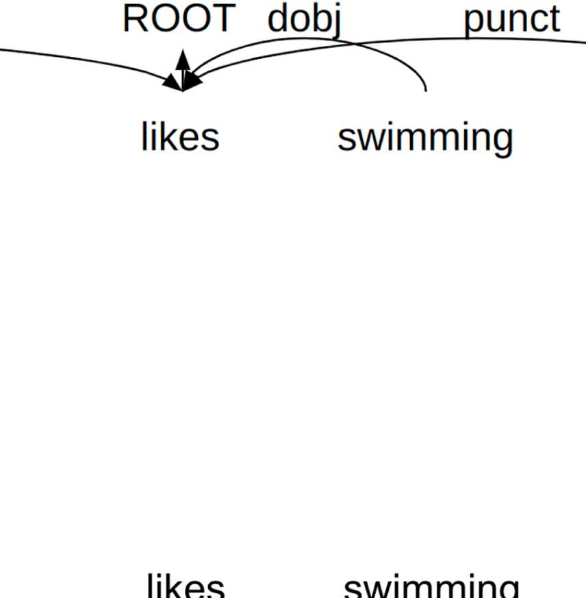
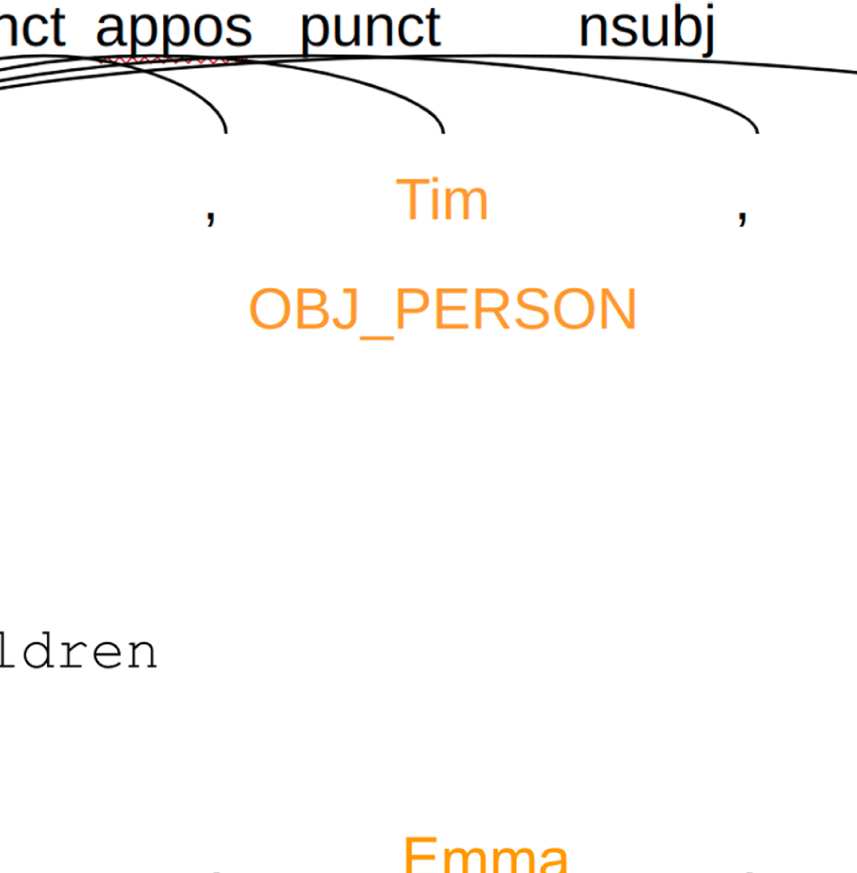
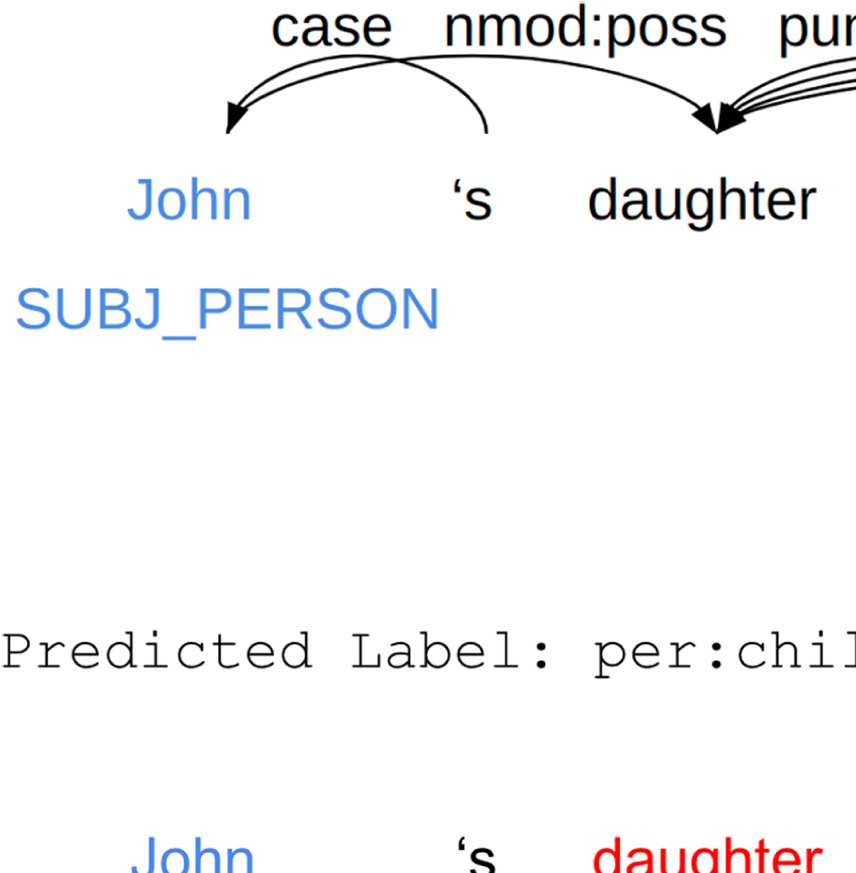
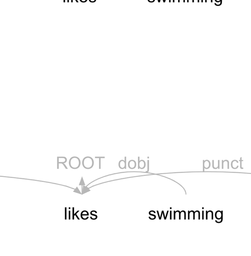
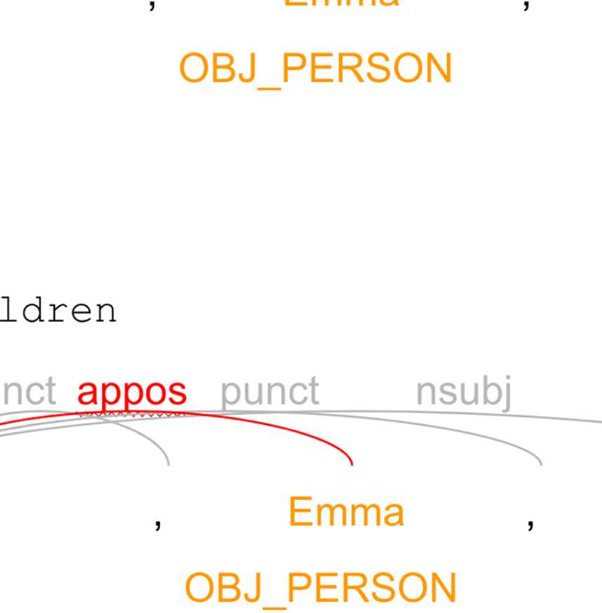
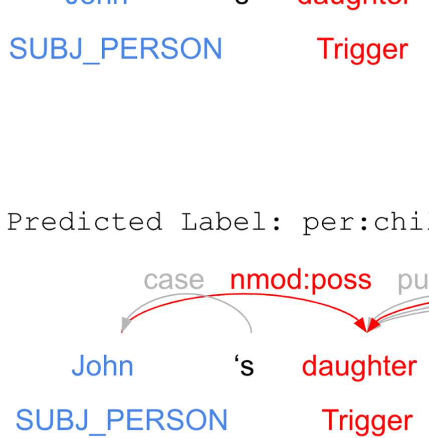
Consider the sentence “John’s daughter, Emma,

likes swimming.”. As shown in
Table 1(a), the task input includes: the raw text in the sentence, the entities participating
in the relation (denoted as subject and object) and their types (PERSON here), and the
syntactic dependency parse tree. Table 1 (b) shows the output of our RC and EC: The
RC returns the predicted relation per:children, while the EC labels the word daughter
as the trigger of the predicted relation. Step (c) shows the information that is collected
for rule generation. This information includes: the two entities, the relation predicted,
the tokens identiﬁed by the EC as the rationale for the relation, and the shortest syntactic
path connecting the two entities with the rationale words. The output rule generated by
our approach is shown in step (d). This rule is written in the Odin language (Valenzuela-
Esc´arcega et al. 2015; Valenzuela-Esc´arcega, Hahn-Powell, and Surdeanu 2016). The
rule captures the relation to be predicted (per:children), its trigger (daughter), the two
arguments and their type (e.g., subject with the type SUBJ Person), and the syntactic
paths between each argument and the trigger phrase (e.g., nmod:poss for the subject
argument). Note that in this simple example, the trigger consists of a single word, but,
in general, an Odin rule can take any arbitrary sequence of words as its trigger.

This example shows that our method can be deployed in two ways. First, one can
use the joint RC and EC neural classiﬁers, which predict relations that hold between
pairs of entities, as well as local explanations (or rationales) that explain the prediction.
Alternatively, a different class of users may use the output of step (d), which, once
applied on large text collections, contains a set of rules that describes multiple relation

123

D
o
w
n
o
a
d
e
d

f
r
o
m
h

t
t

:
/
/

d
i
r
e
c
t
.

i
t
.

e
d
u
/
c
o

l
i
/

a
r
t
i
c
e
–
p
d

f
/

4
9
1
1
1
7
2
0
6
8
9
6
2
/
c
o

l
i

_
a
_
0
0
4
6
3
p
d

b
y
g
u
e
s
t

o
n
0
7
S
e
p
e
m
b
e
r
2
0
2
3

Computational Linguistics

Volume 49, Number 1

Table 1
Walkthrough example of our approach. The task input includes information about the entities
participating in the relation (denoted as subject and object) and their types (PERSON here). Our
neural architecture, which includes both a relation and explanation classiﬁer, predicts the
relation that holds between the two entities (per:children here, i.e., the object is the child of the
subject), as well as which words best explain the decision (in red). In step (c), the rule generator
collects the necessary information from the annotated sentence, i.e., the shortest syntactic
dependency path that connects the two entities with the explanation words (in red in the ﬁgure).
Step (d) shows the generated rule in the Odin language.

D
o
w
n
o
a
d
e
d

f
r
o
m
h

t
t

:
/
/

d
i
r
e
c
t
.

i
t
.

e
d
u
/
c
o

l
i
/

a
r
t
i
c
e
–
p
d

f
/

4
9
1
1
1
7
2
0
6
8
9
6
2
/
c
o

l
i

_
a
_
0
0
4
6
3
p
d

b
y
g
u
e
s
t

o
n
0
7
S
e
p
e
m
b
e
r
2
0
2
3

classes. This usage may be preferred in real-world situations that have to mitigate the
“technical debt” of neural methods, that is, reduce the cost of maintaining these models
over time (Sculley et al. 2015). Although not within the scope of this work, other works
have shown that rule-based methods for IE can be improved and maintained at a low
cost (Valenzuela-Esc´arcega et al. 2016).

124

Tang and Surdeanu

Multitask Learning of Neural Relation and Explanation Classiﬁers

D
o
w
n
o
a
d
e
d

f
r
o
m
h

t
t

:
/
/

d
i
r
e
c
t
.

i
t
.

e
d
u
/
c
o

l
i
/

a
r
t
i
c
e
–
p
d

f
/

4
9
1
1
1
7
2
0
6
8
9
6
2
/
c
o

l
i

_
a
_
0
0
4
6
3
p
d

b
y
g
u
e
s
t

o
n
0
7
S
e
p
e
m
b
e
r
2
0
2
3

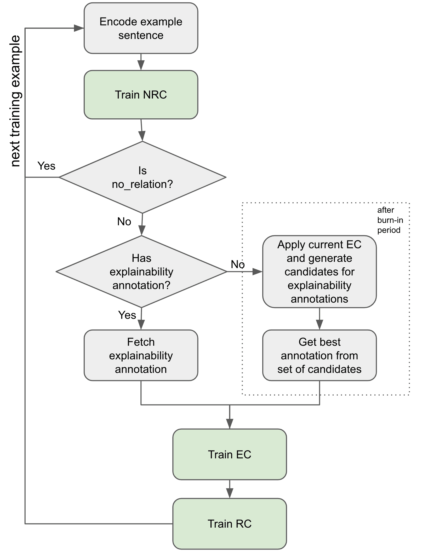
Figure 1
Flow of our semi-supervised training procedure for an individual training example. All the
“Train . . . ” blocks (green background) involve parameter updates of the corresponding
classiﬁers. These updates are shown here for an individual training example, but are batched in
the actual implementation.

3.2 Joint Relation and Explainability Classiﬁers

As mentioned, our approach jointly trains an EC and an RC. The RC is a multiclass
classiﬁer that distinguishes between actual relation labels seen in training. We couple
the RC with a binary classiﬁer that ﬁrst predicts if the current example contains an
actual relation or no relation (marked as no relation). For conciseness, we call this
classiﬁer the no relation classiﬁer (NRC). The EC is a binary word-level classiﬁer, which
labels words in the sentence that contain the relation with 1, if they are important for
the underlying relation, or 0, otherwise.

We start this section with the description of the overall training procedure, and

follow with details about the individual classiﬁers.

3.2.1 Training Procedure. The overall ﬂow of the training procedure is shown in Figure 1.
This ﬂow is temporally split in two periods: a burn-in period, which is fully supervised,

125

Computational Linguistics

Volume 49, Number 1

followed by a period that includes semi-supervised learning (SSL). This distinction is
necessary because while all training examples in this task are guaranteed to have RC
labels, most examples will not have gold explainability annotations. For example, for
the sentence “[CLS] John was born in London.”, the training data contains information
that there is a per:city of birth relation between John and London, but may not contain
information about which words are critical for this relation (born and in).

Burn-in Period. In this stage, shown in the left-hand side of Figure 1, we only use the
training examples that are associated with explainability annotations (see Section 3.2.2
for details on how these annotations are generated). Here we train initial versions of the
three classiﬁers: NRC, EC, and RC (see Section 3.2.3 for details on the three classiﬁers).
The purpose of this stage is to initialize the three classiﬁers such that they can be
successfully used to reduce the search space for explainability annotations in the next
SSL stage.

After burn-in. In this stage, the training procedure is exposed to all training examples, in-
cluding those without annotations for explainability. That is, for such training examples,
we simply have annotations for the relation labels (or no relation), without knowing
which context words explain the underlying relation. In such situations, the right-hand
side of the ﬂow in Figure 1 is used, which triggers two additional components: one to
generate candidates for explainability annotations, and one to choose the best sequence
of word labels (i.e., which words are important and which are not).

For the former component, exhaustively generating all possible label assignments
is prohibitively expensive (i.e., O(2N ) for a sequence of length N). To mitigate this cost,
we rely on the prediction scores of the EC to reduce the number of candidates. That
is, if the score of the binary EC for a given token is higher than a threshold (tup), we
directly annotate the corresponding token as important (i.e., assign label 1); if this score
is lower than a second threshold (tlow), we annotate the token as not important (label 0);
and, lastly, if the the score is between the two thresholds, we generate two candidate
labels for this token (both 0 and 1). For example, given an input sentence “[CLS] [SUBJ-
PER] was born in [OBJ-CITY] .”,1 and these prediction scores from the EC: [0.12,
0.14, 0.19, 0.86, 0.25, 0.15, 0.01], using tup = 0.8 and tlow = 0.2, we produce
the following candidate label sequences: [0, 0, 0, 1, 0, 0, 0] and [0, 0, 0, 1,
1, 0, 0], because the assignment for the token in is ambiguous according to the two
thresholds.

Once these candidates are generated, we loop through all the generated sequences
of word labels, and pick the sequence ˆc that yields the highest score for the correct
relation label according to the current RC:

ˆc = argmax

p(R|c)

(1)

where R is the gold label of the instance, p(R|c) is the score at the gold label R predicted
by the RC for a given annotation candidate c. In the previous example, if the RC scores
of the two candidates for the correct relation label per:city of birth are 0.8 and 0.5,
we select the ﬁrst candidate over the second one.

1 The entities participating in a relation are masked with their named entity labels (see Section 3.2.3).

126

D
o
w
n
o
a
d
e
d

f
r
o
m
h

t
t

:
/
/

d
i
r
e
c
t
.

i
t
.

e
d
u
/
c
o

l
i
/

a
r
t
i
c
e
–
p
d

f
/

4
9
1
1
1
7
2
0
6
8
9
6
2
/
c
o

l
i

_
a
_
0
0
4
6
3
p
d

b
y
g
u
e
s
t

o
n
0
7
S
e
p
e
m
b
e
r
2
0
2
3

Tang and Surdeanu

Multitask Learning of Neural Relation and Explanation Classiﬁers

Then this sequence of labels is used as (pseudo) gold data to train the EC on this
training example. This guarantees that each training example has annotations (gold, or
generated through the above procedure) for both EC and RC.

Because these two components rely on having reasonable predictions from the EC
and RC classiﬁers, we found it beneﬁcial to include the previous burn-in period, where
these classiﬁers are trained using the (small) amount of supervision available.

3.2.2 Explainability Annotation. As mentioned, a key part of our approach requires that
EC annotations be available for a few of the training examples. To this end, rather than
relying on manual annotations, which are expensive, we repurpose rules that extract
the same relation. The intuition behind our approach is that if a rule exists that extracts
the same relation label as the gold label in a training example, then this rule (and,
speciﬁcally, its lexical elements) can be seen as an explanation of the extraction. In
particular, in this article we focus on the TACRED dataset (Zhang et al. 2017), and select
explanations from two sets of rules:

(1) Surface rules: The TACRED project generated a set of high-precision rules for
the task, implemented in the Tokensregex language (Chang and Manning 2014). For
example, the rule SUBJ-PER was born in * OBJ-CITY2 extracts a per:city of birth
relation between a person named entity (the subject) and a city named entity (the object)
if the sequence was born in occurs somewhere between the two entities. For such rules,
we label all tokens contained in the rule (e.g., was, born, in) with the label 1 (i.e., they are
important for explainability), and all other tokens in the sentence with 0.

(2) Syntactic rules: In initial experiments, we observed that the TACRED surface
rules have high precision but low recall. To improve generalization, we also wrote 38
syntax-based rules using the Odin language (Valenzuela-Esc´arcega, Hahn-Powell, and
Surdeanu 2016).3 Figure 2 shows an example of such a rule. For these syntactic rules, we
marked all their lexical elements (typically the trigger predicates such as work or write
in the ﬁgure) as important (label 1), and all other words as not important (label 0).

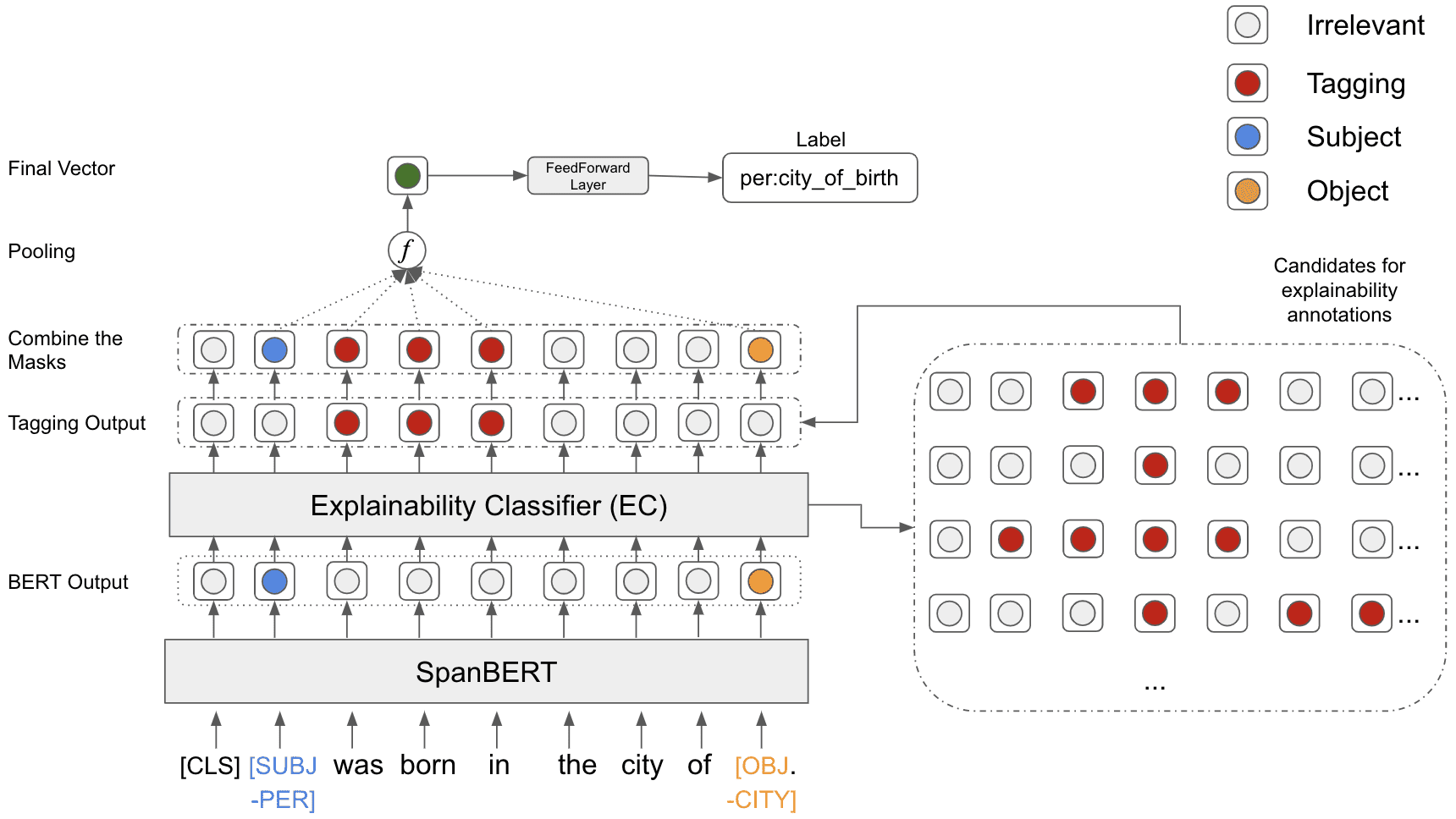
3.2.3 Classiﬁers. As mentioned, the building blocks of our approach consist of three clas-
siﬁers: the no-relation classiﬁer (NRC), the relation classiﬁer (RC), and the explainability
classiﬁer (EC). These are jointly trained using the schema previously described in this
section. Below we describe their individual details, which are also visualized in Figure 3.

SpanBERT Encoder and NRC. We follow the entity masking schema from Zhang et al.
(2017) and replace the subject and object entities with their provided named entity (NE)
labels, for example, “[CLS] [SUBJ-PER] was born in [OBJ-CITY] . . . ”. We feed this input
to a SpanBERT-based (Joshi et al. 2020) encoder:

[hhh0, . . . , hhhn] = Encoder([w0, . . . , wn])

(2)

2 We simpliﬁed the Tokensregex syntax for readability.
3 All these rules are included in this submission as supplemental material available at

https://github.com/clulab/releases/cl2022-twoflints/.

127

D
o
w
n
o
a
d
e
d

f
r
o
m
h

t
t

:
/
/

d
i
r
e
c
t
.

i
t
.

e
d
u
/
c
o

l
i
/

a
r
t
i
c
e
–
p
d

f
/

4
9
1
1
1
7
2
0
6
8
9
6
2
/
c
o

l
i

_
a
_
0
0
4
6
3
p
d

b
y
g
u
e
s
t

o
n
0
7
S
e
p
e
m
b
e
r
2
0
2
3

Computational Linguistics

Volume 49, Number 1

Figure 2
An example of a relation extraction rule in the Odin language that extracts the per:employee of
relation relation. The rule is driven by verbal triggers such as work, play, or serve. The relation’s
arguments (the subject and object) are identiﬁed through both semantic constraints (subject must
be Person), and syntactic ones (subject must be attached to the trigger through a certain syntactic
dependency pattern: an optional (?) adnominal clause (acl), followed by a nominal subject
(nsubj). This rule would extract a per:employee of relation from the text “. . . Joe is a research
scientist working at IBM. . . ”.

D
o
w
n
o
a
d
e
d

f
r
o
m
h

t
t

:
/
/

d
i
r
e
c
t
.

i
t
.

e
d
u
/
c
o

l
i
/

a
r
t
i
c
e
–
p
d

f
/

4
9
1
1
1
7
2
0
6
8
9
6
2
/
c
o

l
i

_
a
_
0
0
4
6
3
p
d

b
y
g
u
e
s
t

o
n
0
7
S
e
p
e
m
b
e
r
2
0
2
3

Figure 3
Neural architecture of the proposed multitask learning approach. The entity tokens (subject in
blue and object in orange) are masked with their named entity labels, e.g., SUBJ-Person, in the
actual implementation.

where wn is the id of the word at position n, and hn is the hidden representation gen-
erated by the encoder. We add the special masking tokens for SUBJ–* and OBJ–* to
the vocabulary so that the encoder can handle them properly. We implement the NRC
using a feedforward layer with a sigmoid function on top of the encoder’s [CLS] token.

128

Tang and Surdeanu

Multitask Learning of Neural Relation and Explanation Classiﬁers

Explainability Classiﬁer (EC). We implement the EC as a binary token-level classiﬁer,
where the positive label indicates that the corresponding token is important for the
underlying relation. Section 3.2.2 discusses how these annotations are generated from
rules; Section 3.2.1 explains the SSL training procedure when these annotations are
not available.

Relation Classiﬁer (RC). Crucially, the RC relies only on words that are marked as impor-
tant by the EC, or are part of the subject/object entity. This is an important distinction
between our approach and other relation extraction methods, which typically rely on
the [CLS] representation for classiﬁcation. In the next section, we empirically show
that this latter strategy is considerably less explainable than ours. This is because the
[CLS] representation aggregates information from all tokens in the sentence, whereas
our method focuses only on the important ones.

We build the aggregated representation of the important context words, subject, and

object as follows:

hhhfinal = f (hhhctx1:ctxn ) ◦ f (hhhsubj1:subjn ) ◦ f (hhhobj1:objn )

(3)

where hhh denotes the hidden representations produced by the encoder, f : Rd×n → Rd is
the average pooling function that maps from n output vectors into one; and ◦ is the
concatenation operator. Importantly, hhhctx iterates only over words marked as important
by the EC.

The concatenated representation hhhfinal is fed to a feedforward layer with a softmax

function to produce a probability distribution ppp over relation types.

The three classiﬁers are trained using the following joint loss function:

loss = lossnrc + lossec + lossrc

lossnrc = −(tn ∗ log(yn) + (1 − tn) ∗ log(1 − yn))
lossec = −(te ∗ log(ye) + (1 − te) ∗ log(1 − ye))
lossrc = −log(p(R))

(4)

(5)

(6)

(7)

where the losses of the NRC and EC (lossnrc and lossec, respectively) are implemented
using binary cross entropy. For both, t indicates the corresponding gold label, and y
is the respective sigmoid’s activation. The loss of the RC (lossrc) is implemented using
categorical cross entropy, where p(R) is the likelihood predicted by the model for the
correct relation R.

3.3 Aggregating Local Explanations into a Global, Rule-based Model

As mentioned, the last component of our approach aggregates all local RC and EC
predictions into a single rule-based model that explains the overall behavior of the RC
and EC models. As such, the produced rule-based model brings global explainability
to the task. We will show in Section 4 that this transformation comes with a cost in
performance, but this cost might be acceptable in scenarios where such RE extraction
must be deployed, maintained, and improved over a long period of time.

129

D
o
w
n
o
a
d
e
d

f
r
o
m
h

t
t

:
/
/

d
i
r
e
c
t
.

i
t
.

e
d
u
/
c
o

l
i
/

a
r
t
i
c
e
–
p
d

f
/

4
9
1
1
1
7
2
0
6
8
9
6
2
/
c
o

l
i

_
a
_
0
0
4
6
3
p
d

b
y
g
u
e
s
t

o
n
0
7
S
e
p
e
m
b
e
r
2
0
2
3

Computational Linguistics

Volume 49, Number 1

Algorithm 1 Rule Generator
Input: set of annotated sentences, S
Input: model output L (from RC) and T (from EC)
1: R ← ∅
2: for every sentence s in S do
3:
4:
5:
6:
7:
8:

Get the subject and object entity es and eo from s
Get the predicted relation label l from L and the rationale words t from T
if s hasn’t been extracted by any manual rule then

Find the shortest path ps between t and es in the dependency tree
Find the shortest path po between t and eo in the dependency tree
r ← empty Odin rule template
Assign l to r as the label to match
Assign t to r as the relation predicate (or trigger)
Assign ps and po to r as the argument patterns.
R ← R ∪ {r}

9:
10:
11:
12:
13:
14: end for
Output: set of generated rules R

end if

3.3.1 Rule Generation. As shown in Table 1(c), our relation and explanation classiﬁers
produce all the information necessary to generate an Odin rule. At a high-level, the
Odin rules we use here follow a predicate (or trigger in the Odin language) and
argument template, where all arguments are connected to the trigger using a syntactic
dependency path. This information is either provided by our classiﬁers (e.g., we use
the rationale tokens identiﬁed by the EC as triggers), or can be automatically extracted
from the sentence (e.g., we represent the syntactic connections between predicate and
arguments using the shortest path that connects them in the syntactic dependency tree).
Algorithm 1 describes this entire rule generation process:

4. Experimental Results

4.1 Data Preparation

We report results on the TACRED dataset (Zhang et al. 2017) and CoNLL04 dataset
(Roth and Yih 2004). As discussed in Section 3.2.2, we provided rules for explanation
supervision. For the TACRED data, we selected rules from the surface patterns of Angeli
et al. (2015), and we combined them with an additional set of 38 syntactic rules in
the Odin language (Valenzuela-Esc´arcega, Hahn-Powell, and Surdeanu 2016) that were
manually created by one of the authors from the training data. For CoNLL04 data, we
selected from a set of 19 syntactic rules in Odin language, 10 of which are borrowed from
the TACRED syntactic rules, since the two datasets shared some overlapping relations.
These rules match 20.7% of positive examples in the TACRED training set and 24.2%
of positive examples in the CoNLL04 training set. On average, 7.27 rules are assigned
to each TACRED relation, and 3.8 rules are assigned to each CoNLL04 relation.

Importantly, our approach does not use rules at evaluation time. However, we take
advantage of all existing rules to automatically evaluate the quality of the explanations

130

D
o
w
n
o
a
d
e
d

f
r
o
m
h

t
t

:
/
/

d
i
r
e
c
t
.

i
t
.

e
d
u
/
c
o

l
i
/

a
r
t
i
c
e
–
p
d

f
/

4
9
1
1
1
7
2
0
6
8
9
6
2
/
c
o

l
i

_
a
_
0
0
4
6
3
p
d

b
y
g
u
e
s
t

o
n
0
7
S
e
p
e
m
b
e
r
2
0
2
3

Tang and Surdeanu

Multitask Learning of Neural Relation and Explanation Classiﬁers

generated by our method. In the TACRED dataset, the combined set of rules from
Angeli et al. (2015) and our syntactic rules match 23.9% of the data points in the
development set, and 23.9% of the examples in the test set; in the CoNLL04 dataset, the
syntactic rules match 20.1% of examples in the development set and 20.9% of examples
in the test set. We use only these matches for an automated evaluation of explainability
(discussed below).

4.2 Baselines

4.2.1 Relation Extraction Baselines. For the relation extraction task, we compare our
approach with three baselines: an extended version of the rule-based approach
of Angeli et al. (2015), a neural state-of-the-art RE approach based on SpanBERT
(Joshi et al. 2020), and a neural approach with built-in explainability (Lei, Barzilay, and
Jaakkola 2016):

•

Rule-based Extraction. As mentioned in Section 4.1, we use two sets of
rules. First, we use the tokensregex surface rules from Angeli et al. (2015),
which are executed in the Stanford CoreNLP pipeline (Manning et al.
2014a). Second, we include the Odin syntactic rules we developed
in-house, which are executed in the Odin framework
(Valenzuela-Esc´arcega, Hahn-Powell, and Surdeanu 2016).4

SpanBERT. SpanBERT (Joshi et al. 2020) is an extension of the original
BERT (Devlin et al. 2018) that: (1) masks continuous random spans
instead of random tokens, and (2) trains the span boundary
representations to predict the full content of the masked span without
depending on individual token representations within it. SpanBERT
outperforms BERT in many tasks including relation extraction. Further,
SpanBERT is currently the best TACRED BERT-based model available in
the HuggingFace transformer library (Wolf et al. 2020) that does not use
any external resources, or does not rely on complex hybrid architectures.

Unsupervised Rationale. Lei, Barzilay, and Jaakkola (2016) proposed an
approach that combines an unsupervised rationale generator with a
task-speciﬁc classiﬁer, both of which are trained to operate together
(similar to our approach). However, there are several key differences
between their method and ours. First, their explanation generator cannot
incorporate human input (as we do through rules); instead, it is indirectly
guided by the loss of the downstream task. Second, their architecture is
more complex, that is, they use two distinct encoders: one for explanation
generation and another for the downstream task (both of which are
implemented with recurrent networks). We adapt this method to our RE
framework, by replacing our EC with their rationale generation
algorithm (which is a token-level binary classiﬁer that produces an
output compatible with our EC). For a fair comparison with our method,

4 The rule set from Angeli et al. (2015) also included some syntactic rules, but we found that they only

matched the simpler per:title relation, so we did not use them.

D
o
w
n
o
a
d
e
d

f
r
o
m
h

t
t

:
/
/

d
i
r
e
c
t
.

i
t
.

e
d
u
/
c
o

l
i
/

a
r
t
i
c
e
–
p
d

f
/

4
9
1
1
1
7
2
0
6
8
9
6
2
/
c
o

l
i

_
a
_
0
0
4
6
3
p
d

b
y
g
u
e
s
t

o
n
0
7
S
e
p
e
m
b
e
r
2
0
2
3

131

Computational Linguistics

Volume 49, Number 1

we kept the other components unchanged. That is, we encode the input
text using the same SpanBERT, then we use their generated rationales
and the given entities as pooling mask to construct the ﬁnal vector to feed
into the relation classiﬁer.5 Originally, Lei, Barzilay, and Jaakkola (2016)
proposed their approach to sentiment analysis and text retrieval.
Bastings, Aziz, and Titov (2019) extended this method and adapted it to a
natural language inference task. To our knowledge, this is the ﬁrst
attempt to apply this explainability strategy to relation extraction.

Note that all baselines as well as our method receive inputs in the standard TACRED
format,6 which contains tokenized sentences, spans of the subject and object mentions,
and the types of the two entity mentions. The only difference between the RC baselines
and our method is that, as discussed in Section 4.1, our approach receives information
on which sentence tokens were matched by rules during the burn-in training period.

4.2.2 Explainability Baselines. For explainability, we compare our approach against eight
baselines, detailed below. These are all popular explanation approaches published in
recent years. Most of them provide a feature importance score for each feature,7 and
most of them are post-hoc.8 Here, we labeled the top N positive features identiﬁed
by the baselines as important.9 In the ﬁrst quantitative evaluation of explainability
(Section 4.4.2), for all baselines we set N to be equal to the number of words in the gold
explanation. Importantly, this means that all baselines have an unfair advantage over
our approach, which is non-parametric with respect to N (i.e., it identiﬁes N on the ﬂy
for each sentence). In the second, qualitative evaluation of explainability (Section 4.4.3),
N is a hyperparameter that we tuned to maximize the baselines’ performance.10

We detail the eight explainability baselines below:

D
o
w
n
o
a
d
e
d

f
r
o
m
h

t
t

:
/
/

d
i
r
e
c
t
.

i
t
.

e
d
u
/
c
o

l
i
/

a
r
t
i
c
e
–
p
d

f
/

4
9
1
1
1
7
2
0
6
8
9
6
2
/
c
o

•

Attention. Attention weights have been proposed as an explanation
mechanism by Bahdanau, Cho, and Bengio (2014). Follow-up work
debated the validity of this strategy (Jain and Wallace 2019; Wiegreffe and
Pinter 2019b; Kobayashi et al. 2020). However, because this remains a
popular approach, we include attention weights as a baseline in this
work. In particular, we use the attention weights from the last layer of a
“vanilla” SpanBERT model, namely, one that is trained on top of the
[CLS] representation, without an EC. For this baseline, we label as
important the top N tokens with the highest [CLS] attention weights.

Saliency Mapping. The feature importance score of the token xi is
determined by the highest prediction’s accumulated gradients in each
dimension of the token in the embedding layer. These scores are obtained

l
i

_
a
_
0
0
4
6
3
p
d

b
y
g
u
e
s
t

o
n
0
7
S
e
p
e
m
b
e
r
2
0
2
3

5 We also observed that our architecture that uses a single, shared transformer encoder performs better

than their original architecture with two distinct encoders.

6 We converted the CoNLL04 data into the same format as TACRED.
7 Except for greedy adding and unsupervised rationale approaches which rely on labeling the features to

be included in the rationale, similar to what we do.

8 Except for unsupervised rationale approach, which trains a generator together with the rest of the model,

similar to what we do.

9 We ignored tokens part of the subject and object entities for a fair comparison.
10 We used N = 3 for TACRED, and N = 1 for CoNLL04.

132

Tang and Surdeanu

Multitask Learning of Neural Relation and Explanation Classiﬁers

through a back-propagation of the highest prediction’s probability.
Although there are different implementations of the gradient saliency
mapping approach (Devlin et al. 2018; Voita, Sennrich, and Titov 2021),
we use the simple back-propagation approach from Simonyan, Vedaldi,
and Zisserman (2013).

LIME. Ribeiro, Singh, and Guestrin (2016) proposed the LIME
framework, which provides explanations to any black-box classiﬁer.
LIME samples the neighbors of the local instance xxx to be explained, by
generating perturbations of the tokens in xxx. Then, it trains a linear
separator from these samples to approximate the local behavior of the
model. The coefﬁcients of the separator are later used as the feature
importance score.

Unsupervised Rationale. As mentioned in the previous sub-section, this
baseline replaces our EC with the unsupervised method of Lei, Barzilay,
and Jaakkola (2016). Here, we use this method as an explainability
baseline.

SHAP. The Shapley value (Shapley 1952) is a cooperative game theory
concept that calculates the score of feature xi by taking into account its
interactions with all other subsets of features. Similar to what LIME does,
Lundberg and Lee (2017) also train a linear model to approximate the
local behavior around the sampled neighbors. However, unlike LIME,
which uses cosine similarity or L2 distance as its kernel, they propose a
SHAP kernel, which is determined by the number of permutations of
features.

CXPlain. Schwab and Karlen (2019) proposed an approach called
CXPlain that explains the decisions of any machine-learning model by
measuring the importance of the model’s features. To this end, CXPlain
masks each token xi in xxx, and calculates the score of xi by comparing the
output with the masked input xxx against the output that relies on the
original input xxx. The difference between the two is calculated using a
causal objective.

Greedy Adding. Instead of randomly sampling from perturbations or
masking the features, Vafa et al. (2021) proposed a method that greedily
adds the features to the input data point. That is, it starts with an empty
rationale, and each time it selects and adds the feature that increases the
probability of the correct label yt the most. The process repeats as long as
the conﬁdence in predicting yt keeps increasing.

All Words between Subject and Object. We have observed that most of
the important words that determine the relation between the entities
occur in the span between the two entities. To capture this intuition, we
implemented this simple baseline, which simply includes all the words
between subject and object in its rationale.

•

Similarly to the RC settings discussed in the previous sub-section, these baselines
and our method rely on the standard TACRED input format. However, our EC is

133

D
o
w
n
o
a
d
e
d

f
r
o
m
h

t
t

:
/
/

d
i
r
e
c
t
.

i
t
.

e
d
u
/
c
o

l
i
/

a
r
t
i
c
e
–
p
d

f
/

4
9
1
1
1
7
2
0
6
8
9
6
2
/
c
o

l
i

_
a
_
0
0
4
6
3
p
d

b
y
g
u
e
s
t

o
n
0
7
S
e
p
e
m
b
e
r
2
0
2
3

Computational Linguistics

Volume 49, Number 1

semi-supervised (i.e., during burn-in it receives explainability annotations generated
by rules). In contrast, the EC baselines do not rely on rule information.

4.3 Implementation and Evaluation Details

Before introducing our results, we discuss key details about our implementation
and evaluation.

To avoid the RC classiﬁer overﬁtting on the names in the sentence (Suntwal
et al. 2019), we mask the subject and object entities by replacing the original tokens
in these entities with a special token, namely, SUBJ– or OBJ–, where
is the corresponding name entity type provided in the dataset. We use the pre-trained
SpanBERT to encode the input sentence. For the TACRED dataset, which is organized to
contain a single relation per sentence, we feed the [CLS] token to the ﬁnal linear layer for
relation classiﬁcation. However, for the CoNLL04 data, which typically contains more
than one relation per sentence, we used the concatenation of the [CLS] hidden state and
the average pooling of [SUBJ] and [OBJ] hidden state embeddings. This was necessary
to distinguish between the different relations that co-occur in the same sentence. We
used the AdamW optimizer (Loshchilov and Hutter 2019) for all training processes. We
evaluated all RC classiﬁers using the standard micro precision, recall, and F1 scores.
All neural models were trained using 5 different random seeds; we report the average
scores and standard deviation over these seeds for RC.

For explainability, we report two evaluations.11 For the ﬁrst, automated evaluation,
we use only the data points that are associated with a rule that produces the same
relation label as the gold data. For these examples, we consider the lexical artifacts
of the rule as gold information for explainability (as explained in §3.2.2). We measure
the overlap between the important words produced by the analyzed methods and
this data using precision, recall, and F1 scores. We also include a second, qualitative
evaluation on the plausability of the generated explanations (Vafa et al. 2021), where
a more plausible explanation will overlap more with a relation explanation manually
generated by domain experts. For this evaluation, we sampled 100 and 60 data points
from the test sets of TACRED and CoNLL04, respectively. These are sentences where
our model predicted a relation, and where there is no gold annotation from the rule-
based method (i.e., no rule matched). We split these data points into two sets: a subset
where our method predicted the correct relation, and one where it did not. In other
words, in the former set, we investigate the capacity of the explainability methods to
explain correct predictions, while in the latter we analyze their capacity to explain why
the machine was incorrect. Two domain experts12 manually annotated rationales for
these sentences and the provided relation labels. The annotators were asked to identify
the minimal set of tokens that explain the provided relation. Or, in other words, identify
the tokens that when replaced with other words change the relation to be predicted.
For example, in the sentence SUBJ-PER was born in OBJ-CITY., if we replace the words
born in with other words (e.g., moved to), the relation between the subject and object
changes. Importantly, to avoid any potential bias, the two annotators worked com-
pletely independently of each other, and had no access to explanations provided by any

11 We did not include an evaluation of faithfulness, which is typically done by post-hoc explainability
approaches (Ribeiro, Singh, and Guestrin 2016; Schwab and Karlen 2019), because our approach is
faithful by design, i.e., our RC only relies on the tokens identiﬁed by the EC.

12 These were two of the authors.

134

D
o
w
n
o
a
d
e
d

f
r
o
m
h

t
t

:
/
/

d
i
r
e
c
t
.

i
t
.

e
d
u
/
c
o

l
i
/

a
r
t
i
c
e
–
p
d

f
/

4
9
1
1
1
7
2
0
6
8
9
6
2
/
c
o

l
i

_
a
_
0
0
4
6
3
p
d

b
y
g
u
e
s
t

o
n
0
7
S
e
p
e
m
b
e
r
2
0
2
3

Tang and Surdeanu

Multitask Learning of Neural Relation and Explanation Classiﬁers

Table 2
Relation extraction results on the TACRED test partition. We used the pre-trained
SpanBERT-large. Our full model trains on the entire training partition using the SSL method
discussed in Section 3.2.1. The “burn-in only” setting trains just on the training subset that has
annotations from rules.

Approach

Rules
SpanBERT (Joshi et al. 2020)
Unsupervised Rationale

Burn-in Only
Full Model

Precision
Baselines

85.82
69.97 ± 0.58
69.24 ± 0.40
Our Approach
51.06 ± 3.57
72.02 ± 0.90

Recall

24.21
70.20
70.20
70.20 ± 1.73
69.05 ± 1.86

37.77
70.07 ± 0.73
69.14 ± 0.83

48.32 ± 2.33
69.11 ± 1.82

49.61 ± 2.42
70.52
70.52 ± 0.54
70.52

algorithm.13 We evaluate the overlap between the machine and human rationales using
the same standard precision, recall, and F1 measures.

Appendix A lists the hyperparameters used to train all RC and EC models.
Lastly, we evaluate the quality of the generated rule-based model. To this end, we
evaluated two sets of rules: rules generated from the training sentences,14 and rules
generated over the test set. In the latter scenario, we do not use any gold data. That is,
we rely on the predicted relation labels (from the RC) and rationales (from the EC) to
generate rules. Thus, the latter setting is akin to transductive learning, that is, where the
model has access to the unlabeled data from the testing partition, but no access to any
human annotations. We evaluate the performance of these rule-based models using the
same micro precision, recall, and F1 scores as the ﬁrst RC evaluation.

D
o
w
n
o
a
d
e
d

f
r
o
m
h

t
t

:
/
/

d
i
r
e
c
t
.

i
t
.

e
d
u
/
c
o

l
i
/

a
r
t
i
c
e
–
p
d

f
/

4
9
1
1
1
7
2
0
6
8
9
6
2
/
c
o

4.4 Results and Discussion

In this section, we introduce and discuss the results for both relation and explainability
classiﬁcation. We conclude this section with an error analysis that highlights some
typical errors in our models.

4.4.1 Relation Extraction. Tables 2 and 3 report the RE performance of all methods dis-
cussed on the TACRED and CoNLL04 datasets. The results of all statistical approaches
are averaged over three random seeds. For all these models we report average perfor-
mance and standard deviation in the tables. We draw the following observations from
these tables:

l
i

_
a
_
0
0
4
6
3
p
d

b
y
g
u
e
s
t

o
n
0
7
S
e
p
e
m
b
e
r
2
0
2
3

•

First, the SSL variant of our approach improves considerably over the
equivalent burn-in only setting (i.e., training just on the data points that
have matching rules). The improvement is 20.91% F1 (absolute) on
TACRED, and 21.83% (absolute) on CoNLL04. These results highlight the
importance of SSL for this task.

13 To encourage reproducibility, we release the annotations at https://github.com/clulab/releases

/tree/master/cl2022-twoflints/dataset.

14 We ﬁlter our training relations which matched a gold rule, since there is already a rule assigned to them.

135

Computational Linguistics

Volume 49, Number 1

Table 3
Relation extraction results on the CoNLL04 test partition. We used the pre-trained
SpanBERT-large. Our full model trains on the entire training partition using the SSL method
discussed in Section 3.2.1. The “burn-in only” setting trains just on the training subset that has
annotations from rules.

Approach

Rules
SpanBERT (Joshi et al. 2020)
Unsupervised Rationale

Burn-in Only
Full Model

Precision
Baselines

81.6
81.30 ± 4.89
83.91
83.91
83.91 ± 2.88
Our Approach
62.71 ± 2.27
83.01 ± 2.16

Recall

16.82
71.01 ± 5.11
74.88 ± 1.44

27.90
75.78 ± 4.79
79.11 ± 1.01

53.32 ± 0.95
76.30
76.30 ± 3.08
76.30

57.63 ± 1.39
79.46
79.46 ± 0.92
79.46

•

Second, our approach is slightly better than SpanBERT on TACRED, and
yields a statistically signiﬁcant improvement of nearly 4% F1 (absolute)
on CoNLL04.15 This indicates that jointly training for classiﬁcation and
explainability helps the classiﬁcation task itself (or, in the worst case, does
not hurt relation classiﬁcation). Table 3 also shows that our approach has
the highest RE recall on CoNLL04, higher than the vanilla SpanBERT by
5%. All in all, this suggests that explainability also serves as a
disambiguator in situations where multiple relations co-occur in the same
sentence (the common setting in CoNLL04) by narrowing the text to just
the context necessary for the relation at hand. As further evidence that
performing RC on top of explanations helps disambiguate the underlying
text, the standard deviation of our approach on CoNLL04 is ﬁve times
smaller than that of SpanBERT.

Interestingly, the unsupervised rationale method approaches the
performance of our full model on both datasets. However, as we will
show in the next sub-section, this comes with considerably worse
explanations.

Lastly, our approach nearly doubles the F1 score of the rule-based
approach on TACRED, and more than doubles it on CoNLL04. This is
caused by large improvements in recall, which highlights the importance
of hybrid strategies that combine rules and neural components.

To understand the runtime overhead introduced by the EC, we compared our
method’s runtimes during training and inference against the runtime of the vanilla
SpanBERT. The average training time of our method is 0.37 sec/batch in the burn-in
period and 0.38 after burn-in. In contrast, the average training time of SpanBERT is 0.06
sec/batch.16 The inference time for both our model and SpanBERT is 0.10 sec/batch
on the same device. The larger overhead in training is caused by: (a) back-propagating

15 We performed statistical signiﬁcance analysis using non-parametric bootstrap resampling with 1,000

iterations.

16 All times measured on an NVIDIA RTX 3090 GPU.

136

D
o
w
n
o
a
d
e
d

f
r
o
m
h

t
t

:
/
/

d
i
r
e
c
t
.

i
t
.

e
d
u
/
c
o

l
i
/

a
r
t
i
c
e
–
p
d

f
/

4
9
1
1
1
7
2
0
6
8
9
6
2
/
c
o

l
i

_
a
_
0
0
4
6
3
p
d

b
y
g
u
e
s
t

o
n
0
7
S
e
p
e
m
b
e
r
2
0
2
3

Tang and Surdeanu

Multitask Learning of Neural Relation and Explanation Classiﬁers

through a larger computational graph due to the joint EC and RC loss, and (b) iterating
through multiple candidate explanations. We measured the average number of expla-
nation candidates to be 85 in the ﬁrst training epoch after burn-in period, and 22 after
10 epochs. However, considering that inference times are similar, we believe that the
training overhead is justiﬁed by the additional explainability functionality included in
the framework.

4.4.2 Quantitative Evaluation of Explainability. The results of the automated evaluation of
explainability in tables 4 and 5 show that our approach generally improves explain-
ability quality considerably. Post-hoc explanation methods do not provide the same
explanation quality compared to our method, which actively models explainability.
Note that the high performance of annotating all the words between subject and object
is caused by the fact that most data points in this evaluation are associated with surface
rules, which prefer shorter contexts that are more likely to contain only signiﬁcant
information. Nevertheless, the 20% F1 gap between this strong baseline and our method
indicates that our method successfully learns how to generalize beyond these simple
scenarios.

However, we note that these results are not terribly surprising: Our method is
trained to generate explanations that mimic lexical artifacts of rules, while the other
explainability baselines have not been exposed to rules during their training. Thus,

D
o
w
n
o
a
d
e
d

f
r
o
m
h

t
t

:
/
/

d
i
r
e
c
t
.

i
t
.

e
d
u
/
c
o

l
i
/

a
r
t
i
c
e
–
p
d

f
/

Table 4
Automated evaluation of explainability on TACRED, in which we compare explainability
annotations produced by these methods against the lexical artifacts of rules.

Approach
Attention
Saliency Mapping
LIME
Unsupervised Rationale
SHAP
CXPlain
Greedy Adding
All words in between SUBJ & OBJ
Our Approach

Precision Recall
30.28
30.22
36.84
79.53
31.27
53.60
50.53
86.33
97.92

30.28
30.22
30.45
4.65
31.27
53.60
40.47
71.48
95.63

F1
30.28
30.22
32.49
8.51
31.27
53.60
40.81
78.21
95.76

Table 5
Automated evaluation of explainability on CoNLL04, in which we compare explainability
annotations produced by these methods against the lexical artifacts of rules.

Approach
Attention
Saliency Mapping
LIME
Unsupervised Rationale
SHAP
CXPlain
Greedy Adding
All words in between SUBJ & OBJ
Our Approach

Precision Recall
69.44
42.42
89.39
86.94
34.85
50.00
54.55
96.59
100

69.44
42.42
62.45
5.47
34.85
50.00
23.24
72.99
99.29

F1
69.44
42.42
68.45
9.84
34.85
50.00
29.58
77.29
99.52

4
9
1
1
1
7
2
0
6
8
9
6
2
/
c
o

l
i

_
a
_
0
0
4
6
3
p
d

b
y
g
u
e
s
t

o
n
0
7
S
e
p
e
m
b
e
r
2
0
2
3

137

Computational Linguistics

Volume 49, Number 1

Table 6
Learning curve of our approach on TACRED based on amount of rules used. In each experiment,
we use up to top k rules per relation type; the number in parentheses is the actual average
number of rules per type.

Num of Rules

Precision Recall

Up to top 1 (0.98 rules/relation)
Up to top 5 (3.56 rules/relation)
Up to top 10 (5.02 rules/relation)
All rules (7.27 rules/relation)

Relation Classiﬁcation
72.48
72.97
69.30
71.15

Explainability Classiﬁcation

Up to top 1 (0.98 rules/relation)
Up to top 5 (3.56 rules/relation)
Up to top 10 (5.02 rules/relation)
All rules (7.27 rules/relation)

74.62
92.19
91.06
95.63

66.23
69.02
71.64
71.13

85.35
94.06
95.62
97.92

69.21
70.94
70.45
71.14

75.02
91.28
91.22
95.76

this evaluation is necessary (to validate that our approach is learning to do what we
intended, which is to mimic the lexical artifacts of rules) but not sufﬁcient. In the next
sub-section, we will show that our approach overlaps with human explanations much
more than all other explainability baselines.

Table 6 lists a learning curve for our approach on TACRED, as we vary the amount
of rules available per relation. That is, for each relation, we use up to top k rules, where
k varies from 1 to 10. In the table we include results for both relation and explainability
classiﬁcation using the same measures as the previous tables. The table shows that
even in the “up to top 5 rules” conﬁguration (which means an average of 3.6 rules per
relation type in practice), our model obtains a close F1 score to our best model with
good explainability. This result indicates that our approach performs well with minimal
human supervision for explanation guidance. Note that we do not include the learning
curve for CoNLL04 since there are only 19 rules applied to this dataset, which translates
into only 3.8 per relation type.

4.4.3 Qualitative Evaluation of Explainability. Tables 7 and 8 list the results of our evalua-
tion of the plausability of explanations by comparing them against human annotations

Table 7
TACRED evaluation of the plausability of explanations, which measures the overlap between
machine explanations and human annotations. For each method, we pick the higher F1 score
between the two human annotators.

Approach
Attention
Saliency Mapping
LIME
Unsupervised Rationale
SHAP
CXPlain
Greedy Adding
Our Approach

Precision Recall
20.60
35.58
26.03
69.66
22.85
55.06
33.52
61.20

41.39
18.73
14.31
4.73
13.86
28.84
31.59
74.72

F1
26.50
23.41
18.09
8.30
16.79
36.48
30.16
62.05

138

D
o
w
n
o
a
d
e
d

f
r
o
m
h

t
t

:
/
/

d
i
r
e
c
t
.

i
t
.

e
d
u
/
c
o

l
i
/

a
r
t
i
c
e
–
p
d

f
/

4
9
1
1
1
7
2
0
6
8
9
6
2
/
c
o

l
i

_
a
_
0
0
4
6
3
p
d

b
y
g
u
e
s
t

o
n
0
7
S
e
p
e
m
b
e
r
2
0
2
3

Tang and Surdeanu

Multitask Learning of Neural Relation and Explanation Classiﬁers

Table 8
CoNLL04 evaluation of the plausability of explanations, which measures the overlap between
machine explanations and human annotations. For each method, we pick the higher F1 score
between the two human annotators.

Approach
Attention
Saliency Mapping
LIME
Unsupervised Rationale
SHAP
CXPlain
Greedy Adding
Our Approach

Precision Recall
30.30
39.39
53.33
74.55
36.36
44.55
38.03
59.24

61.06
18.79
22.14
5.35
18.18
21.21
33.33
65.15

F1
38.94
24.43
30.09
9.31
23.27
27.82
32.21
58.97

of explainability. Similar to evaluations of machine translation, we choose the higher
scores between the machine methods and any of the two human annotators. Note
that the human annotators had a Kappa agreement (McHugh 2012) of 69.8% on
labeling the same tokens as part of an explanation. This is considered moder-
ate (Landis and Koch 1977), which we found encouraging considering the complexity
of the task and the ﬁne granularity of the annotations. We investigated the differences
between the human annotators and observed that they are caused either by legitimate
annotation errors or by the fact that there are multiple valid rationales for a given
relation. For example, in the sentence OBJ-PER is the CEO and president of SUBJ-ORG,
the relation org:top membersemployees can be explained either by the tokens CEO or
president.

The two tables indicate that our approach generates explanations that have consid-
erably higher overlap with human-generated explanations, even though all data points
that are part of this evaluation were chosen to not have a matching rule. This suggests
that our approach generates high-quality explanations of its predictions regardless of
whether it has seen the underlying pattern or not. Moreover, the recall of our approach is
much higher than that of the other post-hoc explanations, which have not been exposed
to rules during training. This shows that with a small amount of supervision, the
generated explanations can be better aligned with human intuitions. The fact that our
method outperforms considerably the unsupervised rationale approach of Lei, Barzilay,
and Jaakkola (2016), which is driven solely by relation classiﬁcation performance, fur-
ther emphasizes that a “human-in-the-loop” method such as ours is necessary to yield
meaningful explanations.

We include several examples of the generated rationales in ﬁgures 4, 5, 6, and 7.
These examples indicate that most of the baselines are noisier, that is, they contain a
considerable amount of false positives (words that should not be part of the rationale)
and false negatives (words that should be included but are not). In contrast, our method
does a better job focusing on the right explanation tokens.

In the example in Figure 4, both our RC model and vanilla BERT predicted the
correct relation. However, our method labels only the preposition of and the determiner
the as its explanation, while other baselines such as LIME and SHAP completely missed
them. Greedy adding and CXPlain label more irrelevant words in the context such as
( and press conference. The attention weights do capture the key words, but we can
clearly see additional noise surrounding the entities. In the example in Figure 5, both

139

D
o
w
n
o
a
d
e
d

f
r
o
m
h

t
t

:
/
/

d
i
r
e
c
t
.

i
t
.

e
d
u
/
c
o

l
i
/

a
r
t
i
c
e
–
p
d

f
/

4
9
1
1
1
7
2
0
6
8
9
6
2
/
c
o

l
i

_
a
_
0
0
4
6
3
p
d

b
y
g
u
e
s
t

o
n
0
7
S
e
p
e
m
b
e
r
2
0
2
3

Computational Linguistics

Volume 49, Number 1

D
o
w
n
o
a
d
e
d

f
r
o
m
h

t
t

:
/
/

d
i
r
e
c
t
.

i
t
.

e
d
u
/
c
o

l
i
/

a
r
t
i
c
e
–
p
d

f
/

4
9
1
1
1
7
2
0
6
8
9
6
2
/
c
o

l
i

_
a
_
0
0
4
6
3
p
d

b
y
g
u
e
s
t

o
n
0
7
S
e
p
e
m
b
e
r
2
0
2
3

Figure 4
Examples of explainability annotations on TACRED for a correct RC prediction. The subject and
object entities, which are provided in the task input, are highlighted in blue and orange. The
important tokens for explainability identiﬁed by the various methods are highlighted in red.
The bottom of the ﬁgure shows the heatmap of [CLS] attention weights for BERT’s 16 heads (the
lighter the color the higher the weight). We shrink the weight range margin to make the color
scale distinguishable. For a fair comparison, we masked the subject and object in the
attention weights.

140

Tang and Surdeanu

Multitask Learning of Neural Relation and Explanation Classiﬁers

D
o
w
n
o
a
d
e
d

f
r
o
m
h

t
t

:
/
/

d
i
r
e
c
t
.

i
t
.

e
d
u
/
c
o

l
i
/

a
r
t
i
c
e
–
p
d

f
/

4
9
1
1
1
7
2
0
6
8
9
6
2
/
c
o

l
i

_
a
_
0
0
4
6
3
p
d

b
y
g
u
e
s
t

o
n
0
7
S
e
p
e
m
b
e
r
2
0
2
3

Figure 5
Examples of explainability annotations on TACRED for an incorrect RC prediction. This ﬁgure
follows the same convention as Figure 4.

our model and the vanilla model predicted the incorrect relation. Our model labels
the preposition for, which provides a strong hint for its (possibly) incorrect prediction
(per:countries of residence). In contrast, the baselines focus more on the nouns
such as defender and champion. Applying the substitution heuristic indicates that the
preposition for is necessary for the explanation (e.g., changing it to against changes the
relation), while the nouns are not relevant. In this example, the attention weights are
almost completely noisy.

In Figure 6, both our model and the vanilla SpanBERT model produce the correct
prediction. The words Secretary-General clearly explain the Work For relation in the

141

Computational Linguistics

Volume 49, Number 1

D
o
w
n
o
a
d
e
d

f
r
o
m
h

t
t

:
/
/

d
i
r
e
c
t
.

i
t
.

e
d
u
/
c
o

l
i
/

a
r
t
i
c
e
–
p
d

f
/

4
9
1
1
1
7
2
0
6
8
9
6
2
/
c
o

l
i

_
a
_
0
0
4
6
3
p
d

b
y
g
u
e
s
t

o
n
0
7
S
e
p
e
m
b
e
r
2
0
2
3

Figure 6
Examples of explainability annotations on CoNLL04 for a correct RC prediction. This ﬁgure
follows the same convention as Figure 4.

explanations generated by our model and greedy adding. The other baselines do not
provide meaningful explanations here. In Figure 7, which shows an incorrect prediction,
only our model can defend its prediction by its explanation. The baseline approaches
cannot provide valid explanations to defend the prediction at all. We also ﬁnd that with
the explanation provided from our model, one can argue that the predicted relation is
actually correct, and we should change the gold label instead.

142

Tang and Surdeanu

Multitask Learning of Neural Relation and Explanation Classiﬁers

D
o
w
n
o
a
d
e
d

f
r
o
m
h

t
t

:
/
/

d
i
r
e
c
t
.

i
t
.

e
d
u
/
c
o

l
i
/

a
r
t
i
c
e
–
p
d

f
/

4
9
1
1
1
7
2
0
6
8
9
6
2
/
c
o

l
i

_
a
_
0
0
4
6
3
p
d

b
y
g
u
e
s
t

o
n
0
7
S
e
p
e
m
b
e
r
2
0
2
3

Figure 7
Examples of explainability annotations on CoNLL04 for an incorrect RC prediction. This ﬁgure
follows the same convention as Figure 4.

Lei, Barzilay, and Jaakkola (2016) state that rationales should be short, coherent,
and be sufﬁcient for the correct prediction. However, short does not necessarily mean
simple. To highlight this point, Figure 8 compares the distribution of POS tags in the
TACRED test partition with the distribution of POS tags that participate in explana-
tions in the same partition. We draw two observations from this data. First, to extract
plausible rationales, our EC has to diverge from the distribution of POS tags in the data
in a non-trivial way. For example, the frequency of verbs (VB*), prepositions (IN), and
commas is considerably higher in the explanations than the raw data. Second, the ﬁgure
indicates that our explanations often focus on parts of speech that are necessary for
plausability (according to the human annotators) but are semantically ambiguous such

143

Computational Linguistics

Volume 49, Number 1

Counts of POS tags in the test partition.

D
o
w
n
o
a
d
e
d

f
r
o
m
h

t
t

:
/
/

d
i
r
e
c
t
.

i
t
.

e
d
u
/
c
o

l
i
/

a
r
t
i
c
e
–
p
d

f
/

4
9
1
1
1
7
2
0
6
8
9
6
2
/
c
o

l
i

_
a
_
0
0
4
6
3
p
d

b
y
g
u
e
s
t

o
n
0
7
S
e
p
e
m
b
e
r
2
0
2
3

Counts of POS tags in the explanations in the test partition.

Figure 8
The distributions of POS tags in the TACRED test partition. The top ﬁgure shows how many
times each POS tag appears in the test data. The bottom ﬁgure shows how many times each POS
tag appears in the generated explanations from the same partition.

as prepositions (IN), commas,17 and determiners (DT). This is different from traditional
pattern acquisition methods (Riloff 1996), which usually focus on words with more clear
semantics such as nominals and verbs.18

17 Commas are necessary to capture appositive constructs, which are often indicative of relations, e.g.,

“Barack Obama, the former president.” In cases such as these, the subject and object of the relation (e.g.,
“Barack Obama” and “former president,” respectively) cover most lexical information relevant to the
relation. In these cases, the remaining signal that indicates the apposition is the comma.

18 Note that traditional patterns may include prepositions and particles, e.g., in verb constructs such as

SUBJECT was born in OBJECT. However, these patterns are usually semantically headed by verb phrases
or nominalized predicates, e.g., born, and seldom by prepositions.

144

Tang and Surdeanu

Multitask Learning of Neural Relation and Explanation Classiﬁers

Table 9
Ablation results on the TACRED test partition, i.e., “–” indicates that the corresponding
component was removed from the full system, and “N/A” indicates that that metric is not
applicable.

Full Model
− NRC
− EC

Vanilla SpanBERT

RC F1
70.52
70.52
70.52 ± 0.54
67.47 ± 0.54
70.62 ± 0.46
70.07 ± 0.73

Quantitative EC F1 Qualitative EC F1

95.76
92.95
N/A
N/A

62.05
54.70
N/A
N/A

Table 10
Ablation results on the CoNLL04 test partition, i.e., “–” indicates that the corresponding
component was removed from the full system, and “N/A” indicates that that metric is not
applicable.

Full Model
− NRC
− EC

Vanilla SpanBERT

RC F1
79.46
79.46
79.46 ± 0.92
77.34 ± 2.33
76.58 ± 1.52
75.78 ± 4.79

Quantitative EC F1 Qualitative EC F1

99.52
99.00
N/A
N/A

58.97
50.12
N/A
N/A

4.4.4 Ablation Study. To understand the impact of the classiﬁers used by our approach
(i.e., NRC, RC, and EC), we implemented ablation experiments on both datasets, which
are summarized in tables 9 and 10. Note that the method without both NRC and
EC becomes equivalent to the vanilla SpanBERT (as we discussed in Section 4.2.1).
Overall, this experiment re-emphasizes that not only does our approach outperform
the vanilla SpanBERT, but it does so while generating an explanation for its decisions.
Removing the NRC drops the relation classiﬁcation F1 score by approximately 3 points
on TACRED, and 2 points on CoNLL04. This impact is explained by the fact that using
the NRC avoids the meaningless scenario where the EC (which was trained only on
positive examples) is applied to negative examples. Interestingly, removing the EC
has no statistical impact on relation classiﬁcation performance on TACRED, but it re-
duces the relation classiﬁcation F1 by approximately 3 points on CoNLL04. As discussed
in Section 4.4.1, this is caused by the fact that the EC serves as a useful disambiguator
in CoNLL04, where multiple relations co-occur in the same sentence. The EC is not that
impactful in TACRED, which has a more artiﬁcial setting with much fewer relations
per sentence.19

4.4.5 Interpretability: From Local to Global. Lastly, we evaluate the performance of our
rule-based model that relies solely on rules, some of which were manually written (see
Section 4.1), while some were automatically generated by our approach, as described in

19 The average number of relations per sentence in TACRED is approximately 2 in training, and 1 in

development and test.

145

D
o
w
n
o
a
d
e
d

f
r
o
m
h

t
t

:
/
/

d
i
r
e
c
t
.

i
t
.

e
d
u
/
c
o

l
i
/

a
r
t
i
c
e
–
p
d

f
/

4
9
1
1
1
7
2
0
6
8
9
6
2
/
c
o

l
i

_
a
_
0
0
4
6
3
p
d

b
y
g
u
e
s
t

o
n
0
7
S
e
p
e
m
b
e
r
2
0
2
3

Computational Linguistics

Volume 49, Number 1

Table 11
Performance of the rule-based model on the TACRED test partition. [1] is the set of manually
written surface rules of Angeli et al. (2015) coupled with our syntactic rules (see Section 4.1). [2]
is the set of rules generated from our explainability classiﬁer’s outputs with gold labels on the
training partition. [3] is the set of rules from the explainability classiﬁer’s outputs with predicted
labels on the test partition. We also evaluate the performance on combinations of these sets of
rules: [2]+[3] contain all rules generated by our approach; [1]+[2]+[3] combine
machine-generated rules with the manually written rules.

Approach

Precision Recall

Baseline

Manual Rules[1]

85.93

24.24

37.81

Our Approach

Rules from Training[2]
Rules from Test[3]
Combination of [1] and [2]
Combination of [1] and [3]
Combination of [2] and [3]
Combination of [1], [2], and [3]

49.39
59.69
54.12
65.28
56.34
57.36

30.26
55.04
62.95
71.64
40.90
72.00

37.52
57.27
58.20
68.31
47.40
63.85

Table 12
Performance of the rule-based model on the CoNLL04 test partition. This table follows the same
conventions as Table 11, except, in this case, [1] is the set of manually written Odin rules we
wrote for CoNLL04.

Approach

Precision Recall

Baseline

Manual Rules[1]

81.82

17.06

28.24

Our Approach

Rules from Training[2]
Rules from Test[3]
Combination of [1] and [2]
Combination of [1] and [3]
Combination of [2] and [3]
Combination of [1], [2], and [3]

66.10
67.95
71.06
68.48
64.01
66.67

27.73
50.24
39.57
59.72
55.21
63.03

39.07
57.77
50.84
63.80
59.29
64.80

Section 3.3. The results are summarized in tables 11 and 12. We draw two observations
from these results:

•

Automatically generated rules can outperform manually written ones.
However, in order to approach the performance of the neural RC, our
method beneﬁts from being aware of the distribution of words in each
testing sentence to be processed (setting [3] in the tables). Importantly, we
reiterate that when using the test sentences, our approach does not have
access to any gold human annotations for RC and EC. That is, the rules
generated from test sentences rely only on predicted relation labels and
predicted explanations for each given sentence. The fact that rules need
to be exposed to more data before they generalize is not extremely
surprising: the rule matching engine we currently use relies on exact

146

D
o
w
n
o
a
d
e
d

f
r
o
m
h

t
t

:
/
/

d
i
r
e
c
t
.

i
t
.

e
d
u
/
c
o

l
i
/

a
r
t
i
c
e
–
p
d

f
/

4
9
1
1
1
7
2
0
6
8
9
6
2
/
c
o

l
i

_
a
_
0
0
4
6
3
p
d

b
y
g
u
e
s
t

o
n
0
7
S
e
p
e
m
b
e
r
2
0
2
3

Tang and Surdeanu

Multitask Learning of Neural Relation and Explanation Classiﬁers

•

lexical matching, which means that the actual tokens to be matched must
be present in the rule. However, the fact that the knowledge necessary to
encode a relation extraction can be encoded into rules is exciting. The
combination of these observations suggests that a future avenue for
research that focuses on “soft rule matching” (Zhou et al. 2020) might be
the direction that captures the advantages of both rules and neural
methods.

Interestingly, automatically generated rules tend to be complementary to
the manual ones. The combination of all three rule sets ([1], [2], and [3] in
the tables) outperforms considerably both the setting that relies solely on
manual rules and the conﬁguration that relies only on automatically
generated ones. The combination of all rule sets outperforms the
manually generated rules by 31% F1 and 38% F1 (absolute) in TACRED
and CoNLL04, respectively. Furthermore, the TACRED result of the
combined rule set approaches the performance of the neural RC within
less than 3% F1. The performance gap between the combined rule set and
neural RC in CoNLL04 is larger (over 14% F1).20 Nevertheless, all in all,
this result suggests that humans and machines can collaborate toward
building a fully explainable model that comes reasonably close to the
performance of neural classiﬁers.

4.4.6 Error Analysis. We conclude this section with a brief error analysis of our explain-
ability classiﬁer in the TACRED and CoNLL04 datasets. Table 13 summarizes a few
typical errors observed in the two datasets.

The ﬁrst two rows in the table show examples where the EC generates explanations
that rely solely on the subject and object entities, without including any word in the
relations’ contexts. Note that the example shown in the ﬁrst row is potentially correct: It
is likely that a location name that immediately precedes an organization name indicates
the location of that organization. However, the second example is clearly incorrect: The
correct explanation to justify the no relation label should minimally include not and
relative. Further, please note that a hypothetical RC that had access to the unmasked
entities could potentially perform even better. For example, in the ﬁrst case, one could
infer that O Globo is based in Rio de Janeiro because the former organization name is
Portuguese. However, our RC only sees masked subjects and objects. Nevertheless,
we believe that our strategy of masking entities participating in relations is a valuable
exercise, as it investigates the capacity of neural methods to identify explicit context
necessary for relation extraction.

Rows 3 and 4 in the table show examples where our RC makes incorrect predictions
due to incorrect tokens labeled by the EC. For example, the token president in row
4 guides the RC toward the incorrect prediction org:top members/employees. The
situation in the third row is more subtle: One might argue that China here can also be
referring to the government, which makes the prediction Work for correct. In any case,
these errors indicate that our explanations can be used for debugging purposes when
the RC makes incorrect predictions.

20 We conjecture that the cause for this larger gap is the lower quality of the rules used for the CoNLL04
dataset. That is, the TACRED rules were developed by a larger team over a longer period of time,
whereas the CoNLL04 rules were developed by one of the authors in only a few hours.

147

D
o
w
n
o
a
d
e
d

f
r
o
m
h

t
t

:
/
/

d
i
r
e
c
t
.

i
t
.

e
d
u
/
c
o

l
i
/

a
r
t
i
c
e
–
p
d

f
/

4
9
1
1
1
7
2
0
6
8
9
6
2
/
c
o

l
i

_
a
_
0
0
4
6
3
p
d

b
y
g
u
e
s
t

o
n
0
7
S
e
p
e
m
b
e
r
2
0
2
3

Computational Linguistics

Volume 49, Number 1

Table 13
Typical errors that our explainability classiﬁer commits. These include errors of under prediction
(ﬁrst two rows), misleading prediction (middle two rows), and errors of over prediction (last two
rows). This ﬁgure follows the same convention as Figure 4.

D
o
w
n
o
a
d
e
d

f
r
o
m
h

t
t

:
/
/

d
i
r
e
c
t
.

i
t
.

e
d
u
/
c
o

l
i
/

a
r
t
i
c
e
–
p
d

f
/

4
9
1
1
1
7
2
0
6
8
9
6
2
/
c
o

The last two rows in the table show examples where our EC over included words
in its explanations. For example, in the last row, a likely interpretation is that the verb is
should be part of the correct explanation, but all the other words are unnecessary. This
happens because the rule lexical triggers in TACRED tend to contain multiple words,
which encouraged the EC to learn to include additional words in its explanation. In
contrast, in CoNLL04 (second to last row), most triggers are single-word phrases. This
prompted the EC to include one token in its explanation, even though it is unnecessary
for the prediction of the relation label in this case.

For a more complete bigger picture, we analyzed the overall frequency of these error
types on the same sampled instances we used for the qualitative explanation evaluation
(Section 4.4.3). Errors where the EC provided no explanations21 occurred in 4.12% of
examples in TACRED, and 19.41% in CoNLL04. Errors where the explanations caused
false positive relations to be predicted appeared 25.95% times in TACRED, and 16.49%
in CoNLL04. Nevertheless, as tables 4, 5, 7, and 8 show, our EC makes considerably
fewer errors than all other explainability methods. There is no reason to believe that its
current errors cannot be ﬁxed with human feedback that would provide a (hopefully
small) number of rules to adjust imperfect explanations.

l
i

_
a
_
0
0
4
6
3
p
d

b
y
g
u
e
s
t

o
n
0
7
S
e
p
e
m
b
e
r
2
0
2
3

21 We included in this category the situations where the explanation was completely empty or it included

only the subject and/or object entity mentions.

148

Tang and Surdeanu

Multitask Learning of Neural Relation and Explanation Classiﬁers

5. Conclusion

We introduced an explainable approach for relation extraction that jointly trains for
prediction and explainability. Our approach uses a multi-task learning framework with
a shared encoder, and jointly trains a classiﬁer for relation extraction with a second
explainability classiﬁer that labels which words in the context of the relation explain
the underlying relation. Further, our method is semi-supervised, as annotations for the
latter classiﬁer are usually not available.

We evaluated the proposed approach on a relation extraction task in two datasets:
TACRED and CoNLL04. Our evaluation showed that, even with minimal supervision
for explanation guidance, our method generates explanations for the relation classiﬁer’s
decisions that are considerably more accurate and plausible than other strong baselines
such as LIME, or relying on attention weights (Simonyan, Vedaldi, and Zisserman 2013;
Bahdanau, Cho, and Bengio 2014; Ribeiro, Singh, and Guestrin 2016; Lundberg and Lee
2017; Schwab and Karlen 2019; Vafa et al. 2021). Further, our results indicated that jointly
training for explainability and prediction improves the prediction task itself, that is, the
relation classiﬁer performs better when it is exposed only to the textual context deemed
important by the explainability classiﬁer.

We also showed that it is possible to convert these local explanations into global
ones. We converted the outputs of our explainability classiﬁer into a set of rules that
globally explains the behavior of the neural relation classiﬁer. Our results showed that
our strategy for generating a rule-based model pushes the performance of rule-based
approaches closer to that of neural methods.

Longer term, we envision our approach being used in an iterative semi-supervised
learning scenario akin to co-training (Blum and Mitchell 1998). That is, the newly
generated rules can be converted to executable rules that can be applied over large,
unannotated texts to generate new training examples for the relation classiﬁer, and vice
versa. Further, our method could potentially beneﬁt from traditional pattern bootstrap-
ping approaches (Riloff 1996; Lin and Pantel 2001), which could reduce the amount
of human supervision necessary by automatically expanding the set of initial patterns
available.

At a higher level, we hope that this work will support meaningful collaborations
between NLP researchers and subject matter experts in other domains (e.g., medical,
legal), who beneﬁt from the output of NLP systems (e.g., large-scale extraction of
biomedical events) but may not understand the intricacies of the neural methods that
underlie these NLP approaches.

We release all code and data behind this work at: https://github.com/clulab/

releases/cl2022-twoflints/.

Appendix A: Experimental Details

We use the dependency parse trees, POS tags, and NER labels as included in the orig-
inal release of the TACRED dataset. All these were generated with Stanford CoreNLP
(Manning et al. 2014b).

We use the pretrained SpanBERT model (Joshi et al. 2020) available in the Hugging-
Face transformer library (Wolf et al. 2020) as our encoder.22 Table A1 shows the hyper-
parameter details for training the neural models for relation classiﬁcation (SpanBERT)

22 https://huggingface.co/SpanBERT/spanbert-large-cased.

149

D
o
w
n
o
a
d
e
d

f
r
o
m
h

t
t

:
/
/

d
i
r
e
c
t
.

i
t
.

e
d
u
/
c
o

l
i
/

a
r
t
i
c
e
–
p
d

f
/

4
9
1
1
1
7
2
0
6
8
9
6
2
/
c
o

l
i

_
a
_
0
0
4
6
3
p
d

b
y
g
u
e
s
t

o
n
0
7
S
e
p
e
m
b
e
r
2
0
2
3

Computational Linguistics

Volume 49, Number 1

Table A1
Hyperparameter details for training the neural models for relation classiﬁcation (for SpanBERT)
and both components (Unsupervised Rationale and our approach). The numbers with ∗ are the
default values from the SpanBERT implementation available at:
https://github.com/facebookresearch/SpanBERT.

Approach
Number of epochs
Learning rate
Dropout rate
Batch size
Max sequence length
Scheduler

SpanBERT Unsupervised Rationale Our Approach
20
1e-5
0.1
32
128

10∗
2e-5∗
0.1∗
32∗
128∗

20
1e-5
0.1
32
128

Linear scheduler with warm up∗

and both relation and explainability classiﬁcation (Unsupervised Rationale and our
approach). Note that we relied mostly on the default hyperparameter values from
SpanBERT, but used a larger number of epochs with a smaller learning rate to ﬁne-
tune the additional explainability component. The Unsupervised Rationale method was
tuned for relation classiﬁcation, which boosted its RC performance (tables 2 and 3), but
negatively impacted its explainability power (tables 4 and 5).

Some of the explainability baselines do not have hyperparameters, including: atten-
tion, saliency mapping, greedy adding, and all words in between. For SHAP, we use all
default settings from the API provided by the authors at https://shap.readthedocs
.io/en/latest/index.html. For LIME, the number of samples we used is 2,000. And
for CXPlain, the explanation model we use is a 2-layers RNN model, with learning rate
of 0.001, dropout rate of 0.2, and trained for 2 epochs.

D
o
w
n
o
a
d
e
d

f
r
o
m
h

t
t

:
/
/

d
i
r
e
c
t
.

i
t
.

e
d
u
/
c
o

l
i
/

a
r
t
i
c
e
–
p
d

f
/

4
9
1
1
1
7
2
0
6
8
9
6
2
/
c
o

Acknowledgments
We thank the reviewers and action editor for
their thoughtful comments and suggestions.
This work was partially supported by the
Defense Advanced Research Projects Agency
(DARPA) under the World Modelers
program, grant #W911NF1810014, and by the
National Science Foundation (NSF) under
grant #2006583. Mihai Surdeanu declares a
ﬁnancial interest in lum.ai. This interest has
been properly disclosed to the University of
Arizona Institutional Review Committee and
is managed in accordance with its conﬂict of
interest policies.

References
Adadi, Amina and Mohammed Berrada.
2018. Peeking inside the black-box: A
survey on explainable artiﬁcial intelligence
(xai). IEEE Access, 6:52138–52160. https://
doi.org/10.1109/ACCESS.2018
.2870052

Angeli, Gabor, Victor Zhong, Danqi Chen, A.
Chaganty, J. Bolton, Melvin Jose Johnson
Premkumar, Panupong Pasupat, S. Gupta,

150

l
i

_
a
_
0
0
4
6
3
p
d

b
y
g
u
e
s
t

o
n
0
7
S
e
p
e
m
b
e
r
2
0
2
3

and Christopher D. Manning. 2015.
Bootstrapped self training for knowledge
base population. Theory and Applications of
Categories.

Arrieta, Alejandro Barredo, Natalia

D´ıaz-Rodr´ıguez, Javier Del Ser, Adrien
Bennetot, Siham Tabik, Alberto Barbado,
Salvador Garc´ıa, Sergio Gil-L ´opez, Daniel
Molina, Richard Benjamins, et al. 2020.
Explainable artiﬁcial intelligence (xai):
Concepts, taxonomies, opportunities and
challenges toward responsible ai.
Information Fusion, 58:82–115. https://
doi.org/10.1016/j.inffus.2019.12.012

Baehrens, David, Timon Schroeter, Stefan
Harmeling, Motoaki Kawanabe, Katja
Hansen, and Klaus-Robert M ¨uller. 2010.
How to explain individual classiﬁcation
decisions. The Journal of Machine Learning
Research, 11:1803–1831.

Bahdanau, Dzmitry, Kyunghyun Cho, and
Yoshua Bengio. 2014. Neural machine
translation by jointly learning to align and
translate. arXiv preprint arXiv:1409.0473.
Bao, Yujia, Shiyu Chang, Mo Yu, and Regina
Barzilay. 2018. Deriving machine attention

Tang and Surdeanu

Multitask Learning of Neural Relation and Explanation Classiﬁers

from human rationales. arXiv preprint
arXiv:1808.09367. https://doi.org
/10.18653/v1/D18-1216

Bastings, Jasmijn, Wilker Aziz, and Ivan

Titov. 2019. Interpretable neural
predictions with differentiable binary
variables. In Proceedings of the 57th Annual
Meeting of the Association for Computational
Linguistics, pages 2963–2977. https://
doi.org/10.18653/v1/P19-1284

B´echet, Fr´ed´eric, Alexis Nasr, and Franck
Genet. 2000. Tagging unknown proper
names using decision trees. In Proceedings
of the 38th Annual Meeting of the Association
for Computational Linguistics, pages 77–84.

Belinkov, Yonatan, Nadir Durrani, Fahim
Dalvi, Hassan Sajjad, and James Glass.
2017. What do neural machine translation
models learn about morphology? In
Proceedings of the 55th Annual Meeting of the
Association for Computational Linguistics
(Volume 1: Long Papers), pages 861–872.
https://doi.org/10.18653/v1/P17
-1080

Chang, Angel X. and Christopher D.

Manning. 2014. Tokensregex: Deﬁning
cascaded regular expressions over tokens.
Stanford University Computer Science
Technical Reports. CSTR, 2:2014.

Craven, Mark and Jude W. Shavlik. 1996.

Extracting tree-structured representations
of trained networks. In Advances in Neural
Information Processing Systems, pages 24–30.

Danilevsky, Marina, Kun Qian, Ranit

Aharonov, Yannis Katsis, Ban Kawas, and
Prithviraj Sen. 2020. A survey of the state
of explainable AI for natural language
processing. In Proceedings of the 1st
Conference of the Asia-Paciﬁc Chapter of the
Association for Computational Linguistics
and the 10th International Joint Conference
on Natural Language Processing,
pages 447–459.

Devlin, Jacob, Ming-Wei Chang, Kenton Lee,

and Kristina Toutanova. 2018. BERT:
Pre-training of deep bidirectional
transformers for language understanding.
arXiv preprint arXiv:1810.04805.

Blum, Avrim and Tom Mitchell. 1998.

Ebrahimi, Javid, Anyi Rao, Daniel Lowd, and

Combining labeled and unlabeled data
with co-training. In Proceedings of the
Eleventh Annual Conference on
Computational Learning Theory,
pages 92–100. https://doi.org/10.1145
/279943.279962

Boros, Tiberiu, Stefan Daniel Dumitrescu,
and Sonia Pipa. 2017. Fast and accurate
decision trees for natural language
processing tasks. In Proceedings of the
International Conference Recent Advances in
Natural Language Processing, RANLP 2017,
pages 103–110. https://doi.org/10
.26615/978-954-452-049-6 016

Brin, Sergey. 1998. Extracting patterns and

relations from the world wide web.
In WebDB, pages 172–183.

Brunner, Gino, Yang Liu, Damian Pascual,
Oliver Richter, Massimiliano Ciaramita,
and Roger Wattenhofer. 2019. On
identiﬁability in transformers. arXiv
preprint arXiv:1908.04211.

Bunescu, Razvan and Raymond Mooney.

2005. A shortest path dependency kernel
for relation extraction. In Proceedings of
Human Language Technology Conference and
Conference on Empirical Methods in Natural
Language Processing, pages 724–731.

Chan, Yee Seng and Dan Roth. 2011.

Exploiting syntactico-semantic structures
for relation extraction. In Proceedings of the
49th Annual Meeting of the Association for
Computational Linguistics: Human Language
Technologies, pages 551–560.

Dejing Dou. 2017. HotFlip: White-box
adversarial examples for text classiﬁcation.
arXiv preprint arXiv:1712.06751. https://
doi.org/10.18653/v1/P18-2006

Feng, Shi, Eric Wallace, Alvin Grissom II,

Mohit Iyyer, Pedro Rodriguez, and Jordan
Boyd-Graber. 2018. Pathologies of neural
models make interpretations difﬁcult. In
Proceedings of the 2018 Conference on
Empirical Methods in Natural Language
Processing, pages 3719–3728.

Fong, Ruth, Mandela Patrick, and Andrea
Vedaldi. 2019. Understanding deep
networks via extremal perturbations and
smooth masks. In 2019 IEEE/CVF
International Conference on Computer Vision
(ICCV), pages 2950–2958. https://doi
.org/10.1109/ICCV.2019.00304
Frosst, Nicholas and Geoffrey Hinton.

2017. Distilling a neural network into
a soft decision tree. arXiv preprint
arXiv:1711.09784.

Ghorbani, Amirata, Abubakar Abid, and

James Zou. 2019. Interpretation of neural
networks is fragile. In Proceedings of the
AAAI Conference on Artiﬁcial Intelligence,
volume 33, pages 3681–3688.

Gunning, David and David Aha. 2019.

Darpa’s explainable artiﬁcial intelligence
(XAI) program. AI Magazine, 40(2):44–58.
https://doi.org/10.1609/aimag
.v40i2.2850

Han, Xiaochuang, Byron C. Wallace, and

Yulia Tsvetkov. 2020. Explaining black box

151

D
o
w
n
o
a
d
e
d

f
r
o
m
h

t
t

:
/
/

d
i
r
e
c
t
.

i
t
.

e
d
u
/
c
o

l
i
/

a
r
t
i
c
e
–
p
d

f
/

4
9
1
1
1
7
2
0
6
8
9
6
2
/
c
o

l
i

_
a
_
0
0
4
6
3
p
d

b
y
g
u
e
s
t

o
n
0
7
S
e
p
e
m
b
e
r
2
0
2
3

Computational Linguistics

Volume 49, Number 1

predictions and unveiling data artifacts
through inﬂuence functions. In Proceedings
of the 58th Annual Meeting of the Association
for Computational Linguistics,
pages 5553–5563. https://doi.org
/10.18653/v1/2020.acl-main.492
Hancock, Braden, Martin Bringmann,

Paroma Varma, Percy Liang, Stephanie
Wang, and Christopher R´e. 2018. Training
classiﬁers with natural language
explanations. In Proceedings of the 56th
Annual Meeting of the Association for
Computational Linguistics (Volume 1,
Long Papers), pages 1884–1895.
https://doi.org/10.18653/v1/P18
-1175, PubMed: 31130772

Hassan, Hany, Ahmed Hassan Awadallah,
and Ossama Emam. 2006. Unsupervised
information extraction approach using
graph mutual reinforcement. In EMNLP,
pages 501–508.

Hearst, Marti A. 1992. Automatic acquisition

of hyponyms from large text corpora.
In COLING 1992 Volume 2: The 14th
International Conference on Computational
Linguistics, pages 539–545. https://
doi.org/10.3115/992133.992154
Hendricks, Lisa Anne, Zeynep Akata,

Marcus Rohrbach, Jeff Donahue, Bernt
Schiele, and Trevor Darrell. 2016.
Generating visual explanations. In
European Conference on Computer Vision,
pages 3–19.

Hewitt, John, Kawin Ethayarajh, Percy

Liang, and Christopher Manning. 2021.
Conditional probing: Measuring usable
information beyond a baseline. In
Proceedings of the 2021 Conference on
Empirical Methods in Natural Language
Processing, pages 1626–1639.
https://doi.org/10.18653/v1/2021
.emnlp-main.122

Hoffmann, Raphael, Congle Zhang, Xiao
Ling, Luke Zettlemoyer, and Daniel S.
Weld. 2011. Knowledge-based weak
supervision for information extraction
of overlapping relations. In Proceedings
of the 49th Annual Meeting of the Association
for Computational Linguistics: Human
Language Technologies, pages 541–550.
Hoover, Benjamin, Hendrik Strobelt, and
Sebastian Gehrmann. 2020. exBERT: A
visual analysis tool to explore learned
representations in Transformers models. In
Proceedings of the 58th Annual Meeting of the
Association for Computational Linguistics:
System Demonstrations, pages 187–196.
https://doi.org/10.18653/v1/2020
.acl-demos.22

152

Jain, Sarthak and Byron C. Wallace. 2019.

Attention is not explanation. arXiv preprint
arXiv:1902.10186.

Jiang, Jing and ChengXiang Zhai. 2007. A

systematic exploration of the feature space
for relation extraction. In Human Language
Technologies 2007: The Conference of the
North American Chapter of the Association for
Computational Linguistics; Proceedings of the
Main Conference, pages 113–120.

Joshi, Mandar, Danqi Chen, Yinhan Liu,
Daniel S. Weld, Luke Zettlemoyer, and
Omer Levy. 2020. SpanBERT: Improving
pre-training by representing and
predicting spans. Transactions of the
Association for Computational Linguistics,
8:64–77. https://doi.org/10.1162
/tacl a 00300

Kambhatla, Nanda. 2004. Combining lexical,

syntactic, and semantic features with
maximum entropy models for information
extraction. In Proceedings of the ACL
Interactive Poster and Demonstration
Sessions, pages 178–181. https://doi.org
/10.3115/1219044.1219066

Karimi, Amir Hossein, Gilles Barthe, Borja

Balle, and Isabel Valera. 2020.
Model-agnostic counterfactual
explanations for consequential decisions.
In Proceedings of the International Conference
on Artiﬁcial Intelligence and Statistics,
pages 895–905.

Kleinberg, Jon M. 1999. Hubs, authorities,

and communities. ACM Computing
Surveys, 31:5. https://doi.org/10.1145
/345966.345982

Kobayashi, Goro, Tatsuki Kuribayashi, Sho

Yokoi, and Kentaro Inui. 2020. Attention is
not only a weight: Analyzing transformers
with vector norms. In Proceedings of the
2020 Conference on Empirical Methods in
Natural Language Processing (EMNLP),
pages 7057–7075. https://doi.org
/10.18653/v1/2020.emnlp-main.574
Landis, J. Richard and Gary G. Koch. 1977.
The measurement of observer agreement
for categorical data. Biometrics, 33:159–174.
https://doi.org/10.2307/2529310,
PubMed: 843571

Lei, Tao, Regina Barzilay, and Tommi
Jaakkola. 2016. Rationalizing neural
predictions. In Proceedings of the 2016
Conference on Empirical Methods in Natural
Language Processing, pages 107–117.
Li, Jiwei, Xinlei Chen, Eduard Hovy, and
Dan Jurafsky. 2016. Visualizing and
understanding neural models in NLP. In
Proceedings of the 2016 Conference of the
North American Chapter of the Association for

D
o
w
n
o
a
d
e
d

f
r
o
m
h

t
t

:
/
/

d
i
r
e
c
t
.

i
t
.

e
d
u
/
c
o

l
i
/

a
r
t
i
c
e
–
p
d

f
/

4
9
1
1
1
7
2
0
6
8
9
6
2
/
c
o

l
i

_
a
_
0
0
4
6
3
p
d

b
y
g
u
e
s
t

o
n
0
7
S
e
p
e
m
b
e
r
2
0
2
3

Tang and Surdeanu

Multitask Learning of Neural Relation and Explanation Classiﬁers

Computational Linguistics: Human Language
Technologies, pages 681–691. https://doi
.org/10.18653/v1/N16-1082

Li, Jiwei, Will Monroe, and Dan Jurafsky.
2016. Understanding neural networks
through representation erasure. ArXiv,
abs/1612.08220.

Lin, Dekang and P. Pantel. 2001. Dirt –

discovery of inference rules from text.
In Proceedings of the Seventh ACM
SIGKDD International Conference on
Knowledge Discovery and Data Mining,
pages 323–328.

Liu, Ninghao, Xiao Huang, Jundong Li, and

Xia Hu. 2018. On interpretation of network
embedding via taxonomy induction. In
Proceedings of the 24th ACM SIGKDD
International Conference on Knowledge
Discovery & Data Mining, pages 1812–1820.
https://doi.org/10.1145/3219819
.3220001

Loshchilov, Ilya and Frank Hutter. 2019.

Decoupled weight decay regularization.
In Proceedings of ICLR.

Lundberg, Scott M. and Su-In Lee. 2017. A
uniﬁed approach to interpreting model
predictions. In I. Guyon, U. V. Luxburg,
S. Bengio, H. Wallach, R. Fergus, S.
Vishwanathan, and R. Garnett, editors,
Advances in Neural Information Processing
Systems 30. Curran Associates, Inc.,
pages 4765–4774.

Manning, Christopher, Mihai Surdeanu, John
Bauer, Jenny Finkel, Steven Bethard, and
David McClosky. 2014a. The Stanford
CoreNLP natural language processing
toolkit. In Proceedings of 52nd Annual
Meeting of the Association for Computational
Linguistics: System Demonstrations,
pages 55–60. https://doi.org/10
.3115/v1/P14-5010

Manning, Christopher D. 2015. Last words:

Computational linguistics and deep
learning. Computational Linguistics,
41(4):701–707. https://doi.org/10
.1162/COLI a 00239

Manning, Christopher D., Mihai Surdeanu,

John Bauer, Jenny Finkel, Steven J.
Bethard, and David McClosky. 2014b. The
Stanford CoreNLP natural language
processing toolkit. In Association for
Computational Linguistics (ACL) System
Demonstrations, pages 55–60. https://doi
.org/10.3115/v1/P14-5010

McHugh, Mary L. 2012. Interrater reliability:

The kappa statistic. Biochemia Medica,
22(3):276–282. https://doi.org
/10.11613/BM.2012.031, PubMed:
23092060

Miller, Scott, Heidi Fox, Lance Ramshaw, and
Ralph Weischedel. 2000. A novel use of
statistical parsing to extract information
from text. In 1st Meeting of the North
American Chapter of the Association for
Computational Linguistics, pages 226–233.
Mintz, Mike, Steven Bills, Rion Snow, and

Dan Jurafsky. 2009. Distant supervision for
relation extraction without labeled data. In
Proceedings of the Joint Conference of the 47th
Annual Meeting of the ACL and the 4th
International Joint Conference on Natural
Language Processing of the AFNLP,
pages 1003–1011. https://doi.org
/10.3115/1690219.1690287

Mohankumar, Akash Kumar, Preksha Nema,
Sharan Narasimhan, Mitesh M. Khapra,
Balaji Vasan Srinivasan, and Balaraman
Ravindran. 2020. Towards transparent
and explainable attention models. In
Proceedings of the 58th Annual Meeting of the
Association for Computational Linguistics,
pages 4206–4216. https://doi.org/10
.18653/v1/2020.acl-main.387

Moschitti, Alessandro. 2006. Making tree
kernels practical for natural language
learning. In 11th Conference of the European
Chapter of the Association for Computational
Linguistics, 8 pages.

Nguyen, Truc Vien T., Alessandro Moschitti,
and Giuseppe Riccardi. 2009. Convolution
kernels on constituent, dependency and
sequential structures for relation
extraction. In Proceedings of the 2009
Conference on Empirical Methods in Natural
Language Processing, pages 1378–1387.
Peters, Matthew E., Sebastian Ruder, and
Noah A. Smith. 2019. To tune or not to
tune? Adapting pretrained representations
to diverse tasks. In Proceedings of the 4th
Workshop on Representation Learning for
NLP (RepL4NLP-2019), pages 7–14.
https://doi.org/10.18653/v1/W19-4302

Poerner, Nina, Benjamin Roth, and Hinrich
Sch ¨utze. 2018. Evaluating neural network
explanation methods using hybrid
documents and morphological agreement.
arXiv preprint arXiv:1801.06422.
https://doi.org/10.18653/v1/P18-1032

Rajani, Nazneen Fatema, Bryan McCann,

Caiming Xiong, and Richard Socher. 2019.
Explain yourself! Leveraging language
models for commonsense reasoning. In
Proceedings of the 57th Annual Meeting of the
Association for Computational Linguistics,
pages 4932–4942. https://doi.org/10
.18653/v1/P19-1487

Rau, Lisa F., Paul S. Jacobs, and Uri Zernik.
1989. Information extraction and text

153

D
o
w
n
o
a
d
e
d

f
r
o
m
h

t
t

:
/
/

d
i
r
e
c
t
.

i
t
.

e
d
u
/
c
o

l
i
/

a
r
t
i
c
e
–
p
d

f
/

4
9
1
1
1
7
2
0
6
8
9
6
2
/
c
o

l
i

_
a
_
0
0
4
6
3
p
d

b
y
g
u
e
s
t

o
n
0
7
S
e
p
e
m
b
e
r
2
0
2
3

Computational Linguistics

Volume 49, Number 1

summarization using linguistic knowledge
acquisition. Information Processing &
Management, 25(4):419–428.
https://doi.org/10.1016/0306
-4573(89)90069-1

Rawal, Kaivalya and Himabindu Lakkaraju.
2020. Beyond individualized recourse:
Interpretable and interactive summaries of
actionable recourses. Advances in Neural
Information Processing Systems, 33.
Ribeiro, Marco Tulio, Sameer Singh, and

Carlos Guestrin. 2016. Why should I trust
you?: Explaining the predictions of any
classiﬁer. In Proceedings of the 22nd ACM
SIGKDD International Conference on
Knowledge Discovery and Data Mining,
pages 1135–1144. https://doi.org
/10.1145/2939672.2939778

Riedel, Sebastian, Limin Yao, and Andrew
McCallum. 2010. Modeling relations and
their mentions without labeled text. In
Joint European Conference on Machine
Learning and Knowledge Discovery in
Databases, pages 148–163. https://doi
.org/10.1007/978-3-642-15939-8 10
Riloff, Ellen. 1996. Automatically generating
extraction patterns from untagged text. In
Proceedings of the National Conference on
Artiﬁcial Intelligence, pages 1044–1049.
Roth, Dan and Wen-tau Yih. 2004. A linear
programming formulation for global
inference in natural language tasks. In
Proceedings of the Eighth Conference on
Computational Natural Language Learning
(CoNLL-2004) at HLT-NAACL 2004,
pages 1–8.

Schwab, Patrick and Walter Karlen. 2019.

CXPlain: Causal explanations for model
interpretation under uncertainty. In
Advances in Neural Information Processing
Systems (NeurIPS), 11 pages.

Sculley, David, Gary Holt, Daniel Golovin,
Eugene Davydov, Todd Phillips, Dietmar
Ebner, Vinay Chaudhary, Michael Young,
Jean-Francois Crespo, and Dan Dennison.
2015. Hidden technical debt in machine
learning systems. Advances in Neural
Information Processing Systems, 28.

Shapley, Lloyd S. 1952. A Value for N-Person

Games. RAND Corporation, Santa Monica,
CA.

Simonyan, Karen, Andrea Vedaldi, and

Andrew Zisserman. 2013. Deep inside
convolutional networks: Visualising image
classiﬁcation models and saliency maps.
arXiv preprint arXiv:1312.6034.

Situ, Xuelin, Ingrid Zukerman, Cecile Paris,
Sameen Maruf, and Gholamreza Haffari.
2021. Learning to explain: Generating

154

stable explanations fast. In Proceedings of
the 59th Annual Meeting of the Association for
Computational Linguistics and the 11th
International Joint Conference on Natural
Language Processing (Volume 1: Long Papers),
pages 5340–5355. https://doi.org
/10.18653/v1/2021.acl-long.415

Srihari, Rohini and Wei Li. 1999. Information
extraction supported question answering.
Technical report, Cymfony Net Inc,
Williamsville, NY. https://doi.org/10
.21236/ADA460042

Srihari, Rohini K. and Wei Li. 2000. A

question answering system supported by
information extraction. In Sixth Applied
Natural Language Processing Conference,
pages 166–172. https://doi.org
/10.3115/974147.974170

Suntwal, Sandeep, Mithun Paul, Rebecca

Sharp, and Mihai Surdeanu. 2019. On the
importance of delexicalization for fact
veriﬁcation. In Proceedings of the 2019
Conference on Empirical Methods in Natural
Language Processing and the 9th International
Joint Conference on Natural Language
Processing (EMNLP-IJCNLP),
pages 3413–3418. https://doi.org
/10.18653/v1/D19-1340

Surdeanu, Mihai, Julie Tibshirani, Ramesh
Nallapati, and Christopher D. Manning.
2012. Multi-instance multi-label learning
for relation extraction. In Proceedings of the
2012 Joint Conference on Empirical Methods
in Natural Language Processing and
Computational Natural Language Learning,
pages 455–465.

Tang, Zheng, Gus Hahn-Powell, and Mihai

Surdeanu. 2020. Exploring interpretability
in event extraction: Multitask learning of a
neural event classiﬁer and an explanation
decoder. In Proceedings of the 58th Annual
Meeting of the Association for Computational
Linguistics: Student Research Workshop,
pages 169–175. https://doi.org
/10.18653/v1/2020.acl-srw.23

Vafa, Keyon, Yuntian Deng, David M. Blei,
and Alexander M. Rush. 2021. Rationales
for sequential predictions. In Empirical
Methods in Natural Language Processing,
pages 10314–10332.

Valenzuela-Esc´arcega, Marco A., Gus
Hahn-Powell, Dane Bell, and Mihai
Surdeanu. 2016. SnapToGrid: From
statistical to interpretable models for
biomedical information extraction. arXiv
preprint arXiv:1606.09604. https://
doi.org/10.18653/v1/W16-2907
Valenzuela-Esc´arcega, Marco A., Gus

Hahn-Powell, and Mihai Surdeanu. 2016.

D
o
w
n
o
a
d
e
d

f
r
o
m
h

t
t

:
/
/

d
i
r
e
c
t
.

i
t
.

e
d
u
/
c
o

l
i
/

a
r
t
i
c
e
–
p
d

f
/

4
9
1
1
1
7
2
0
6
8
9
6
2
/
c
o

l
i

_
a
_
0
0
4
6
3
p
d

b
y
g
u
e
s
t

o
n
0
7
S
e
p
e
m
b
e
r
2
0
2
3

Tang and Surdeanu

Multitask Learning of Neural Relation and Explanation Classiﬁers

Odin’s runes: A rule language for
information extraction. In Proceedings of the
Tenth International Conference on Language
Resources and Evaluation (LREC’16),
pages 322–329.

Valenzuela-Esc´arcega, Marco A., Gus

Hahn-Powell, Thomas Hicks, and Mihai
Surdeanu. 2015. A domain-independent
rule-based framework for event extraction.
In Proceedings of the 53rd Annual Meeting of
the Association for Computational Linguistics
and the 7th International Joint Conference on
Natural Language Processing of the Asian
Federation of Natural Language Processing:
Software Demonstrations (ACL-IJCNLP),
pages 127–132. https://doi.org/10
.3115/v1/P15-4022

Vaswani, Ashish, Noam Shazeer, Niki

Parmar, Jakob Uszkoreit, Llion Jones,
Aidan N. Gomez, Łukasz Kaiser, and Illia
Polosukhin. 2017. Attention Is all you
need. In Advances in Neural Information
Processing Systems, pages 5998–6008.
Voita, Elena, Rico Sennrich, and Ivan Titov.
2021. Analyzing the source and target
contributions to predictions in neural
machine translation. In Proceedings of the
59th Annual Meeting of the Association for
Computational Linguistics and the 11th
International Joint Conference on Natural
Language Processing (Volume 1: Long
Papers), pages 1126–1140. https://
doi.org/10.18653/v1/2021.acl
-long.91

Vu, Ngoc Thang, Heike Adel, Pankaj Gupta,
and Hinrich Sch ¨utze. 2016. Combining
recurrent and convolutional neural
networks for relation classiﬁcation. In
Proceedings of the 2016 Conference of the
North American Chapter of the Association
for Computational Linguistics: Human
Language Technologies, pages 534–539.
https://doi.org/10.18653/v1/N16-1065
Wachter, Sandra, Brent Mittelstadt, and Chris
Russell. 2018. Counterfactual explanations
without opening the black box: Automated
decisions and the GDPR. Harvard Journal of
Law & Technology, 31:841–887. https://doi
.org/10.2139/ssrn.3063289

Wallace, Eric, Jens Tuyls, Junlin Wang, Sanjay
Subramanian, Matt Gardner, and Sameer
Singh. 2019. AllenNLP Interpret: A
framework for explaining predictions of
NLP models. In Empirical Methods in
Natural Language Processing, 6 pages.
https://doi.org/10.18653/v1/D19-3002

Wang, Junlin, Jens Tuyls, Eric Wallace, and
Sameer Singh. 2020. Gradient-based
analysis of NLP models is manipulable.

arXiv preprint arXiv:2010.05419.
https://doi.org/10.18653/v1
/2020.findings-emnlp.24

Wang, Linlin, Zhu Cao, Gerard de Melo, and
Zhiyuan Liu. 2016. Relation classiﬁcation
via multi-level attention CNNs. In
Proceedings of the 54th Annual Meeting of the
Association for Computational Linguistics
(Volume 1: Long Papers), pages 1298–1307.
https://doi.org/10.18653/v1/P16-1123

Wiegreffe, Sarah and Yuval Pinter. 2019a.
Attention is not not explanation. In
Proceedings of the 2019 Conference on
Empirical Methods in Natural Language
Processing and the 9th International Joint
Conference on Natural Language Processing
(EMNLP-IJCNLP), pages 11–20.

Wiegreffe, Sarah and Yuval Pinter. 2019b.
Attention is not not explanation. arXiv
preprint arXiv:1908.04626.

Wolf, Thomas, Lysandre Debut, Victor Sanh,
Julien Chaumond, Clement Delangue,
Anthony Moi, Pierric Cistac, Tim Rault,
R´emi Louf, Morgan Funtowicz, Joe
Davison, Sam Shleifer, Patrick von Platen,
Clara Ma, Yacine Jernite, Julien Plu,
Canwen Xu, Teven Le Scao, Sylvain
Gugger, Mariama Drame, Quentin Lhoest,
and Alexander M. Rush. 2020.
Transformers: State-of-the-art natural
language processing. In Proceedings of the
2020 Conference on Empirical Methods in
Natural Language Processing: System
Demonstrations, pages 38–45.
https://doi.org/10.18653/v1
/2020.emnlp-demos.6

Wu, Shanchan and Yifan He. 2019. Enriching
pre-trained language model with entity
information for relation classiﬁcation. In
Proceedings of the 28th ACM International
Conference on Information and Knowledge
Management, pages 2361–2364. https://
doi.org/10.1145/3357384.3358119
Xu, Yan, Lili Mou, Ge Li, Yunchuan Chen,
Hao Peng, and Zhi Jin. 2015. Classifying
relations via long short term memory
networks along shortest dependency
paths. In Proceedings of the 2015 Conference
on Empirical Methods in Natural Language
Processing, pages 1785–1794.

Yamada, Ikuya, Akari Asai, Hiroyuki
Shindo, Hideaki Takeda, and Yuji
Matsumoto. 2020. Luke: Deep
contextualized entity representations with
entity-aware self-attention. arXiv preprint
arXiv:2010.01057. https://doi.org
/10.18653/v1/2020.emnlp-main.523
Zechner, Klaus. 1997. A literature survey
on information extraction and text

155

D
o
w
n
o
a
d
e
d

f
r
o
m
h

t
t

:
/
/

d
i
r
e
c
t
.

i
t
.

e
d
u
/
c
o

l
i
/

a
r
t
i
c
e
–
p
d

f
/

4
9
1
1
1
7
2
0
6
8
9
6
2
/
c
o

l
i

_
a
_
0
0
4
6
3
p
d

b
y
g
u
e
s
t

o
n
0
7
S
e
p
e
m
b
e
r
2
0
2
3

Computational Linguistics

Volume 49, Number 1

summarization. Computational Linguistics
Program, 22.

Zelenko, Dmitry, Chinatsu Aone, and
Anthony Richardella. 2003. Kernel
methods for relation extraction.
Journal of Machine Learning Research,
3(Feb):1083–1106.

Zeng, Daojian, Kang Liu, Siwei Lai,

Guangyou Zhou, and Jun Zhao. 2014.
Relation classiﬁcation via convolutional
deep neural network. In Proceedings of
COLING 2014, the 25th International
Conference on Computational Linguistics:
Technical Papers, pages 2335–2344.
Zhang, Dongxu and Dong Wang. 2015.

Relation classiﬁcation via recurrent neural
network. arXiv preprint arXiv:1508.01006.
Zhang, Yuhao, Peng Qi, and Christopher D.
Manning. 2018. Graph convolution over
pruned dependency trees improves
relation extraction. In Proceedings of the
2018 Conference on Empirical Methods in
Natural Language Processing,
pages 2205–2215. https://doi.org
/10.18653/v1/D18-1244

Zhang, Yuhao, Victor Zhong, Danqi Chen,

Gabor Angeli, and Christopher D.
Manning. 2017. Position-aware attention
and supervised data improve slot ﬁlling.
In Proceedings of the 2017 Conference on
Empirical Methods in Natural Language
Processing (EMNLP 2017), pages 35–45.
https://doi.org/10.18653/v1/D17-1004

Zhao, Shubin and Ralph Grishman. 2005.
Extracting relations with integrated

information using kernel methods. In
Proceedings of the 43rd Annual Meeting of the
Association for Computational Linguistics
(ACL’05), pages 419–426.

Zhao, Yiyun and Steven Bethard. 2020. How
does BERT’s attention change when you
ﬁne-tune? An analysis methodology and
a case study in negation scope. In
Proceedings of the 58th Annual Meeting of the
Association for Computational Linguistics,
pages 4729–4747. https://doi.org
/10.18653/v1/2020.acl-main.429

Zhou, GuoDong, Jian Su, Jie Zhang, and Min
Zhang. 2005. Exploring various knowledge
in relation extraction. In Proceedings of the
43rd Annual Meeting of the Association for
Computational Linguistics (ACL’05),
pages 427–434.

Zhou, Peng, Wei Shi, Jun Tian, Zhenyu Qi,
Bingchen Li, Hongwei Hao, and Bo Xu.
2016. Attention-based bidirectional long
short-term memory networks for relation
classiﬁcation. In Proceedings of the 54th
Annual Meeting of the Association for
Computational Linguistics (Volume 2: Short
Papers), pages 207–212. https://doi.org
/10.18653/v1/P16-2034

Zhou, Wenxuan, Hongtao Lin, Bill Yuchen
Lin, Ziqi Wang, Junyi Du, Leonardo
Neves, and Xiang Ren. 2020. NERO: A
neural rule grounding framework for
label-efﬁcient relation extraction. In
Proceedings of The Web Conference 2020,
pages 2166–2176. https://doi.org
/10.1145/3366423.3380282

156

D
o
w
n
o
a
d
e
d

f
r
o
m
h

t
t

:
/
/

d
i
r
e
c
t
.

i
t
.

e
d
u
/
c
o

l
i
/

a
r
t
i
c
e
–
p
d

f
/

4
9
1
1
1
7
2
0
6
8
9
6
2
/
c
o