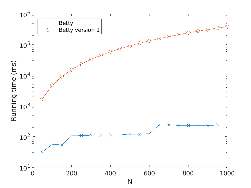
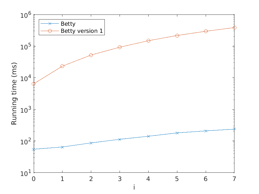
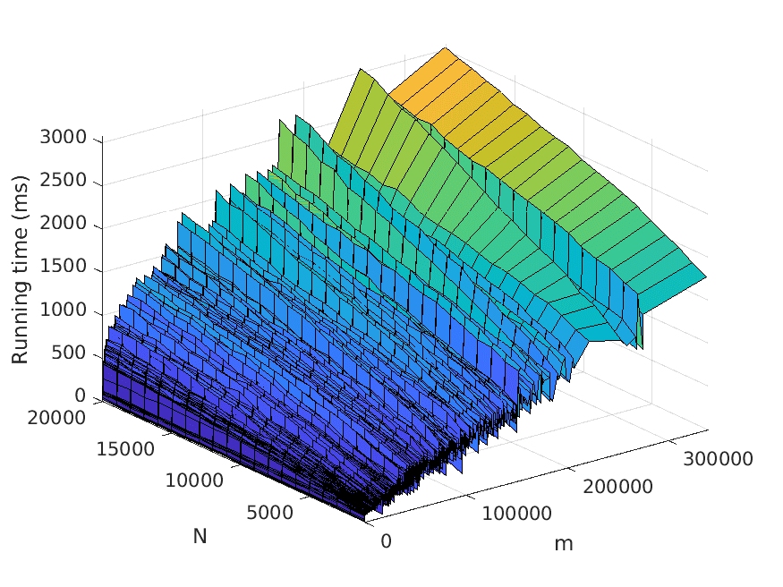
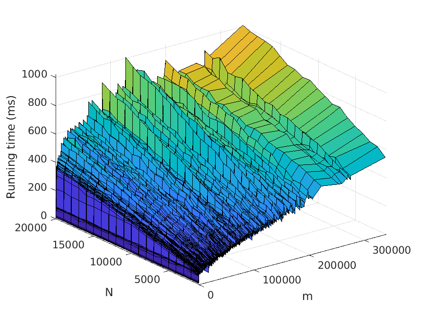
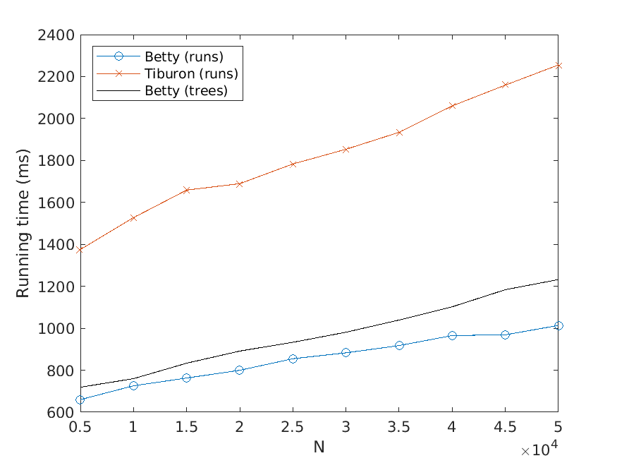
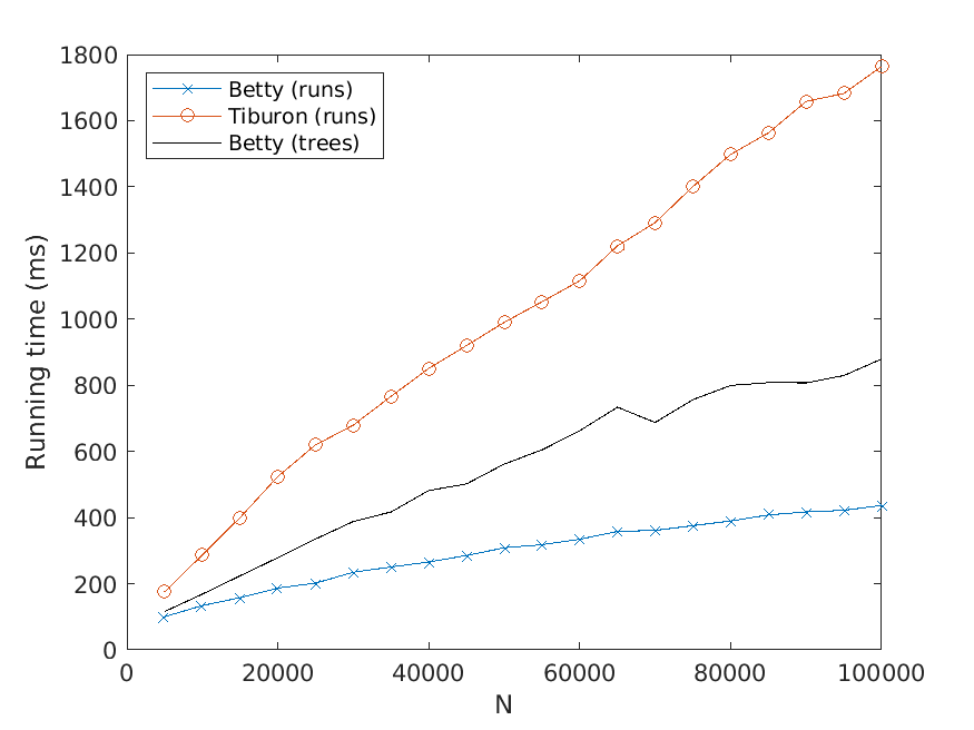
Improved N-Best Extraction with an - Specialized Research AI at MIT

Improved N-Best Extraction with an
Evaluation on Language Data

Johanna Bj ¨orklund
Ume˚a University
Department of Computing Science
johanna@cs.umu.se

Frank Drewes
Ume˚a University
Department of Computing Science
drewes@cs.umu.se

Anna Jonsson
Ume˚a University
Department of Computing Science
aj@cs.umu.se

We show that a previously proposed algorithm for the N-best trees problem can be made more
efﬁcient by changing how it arranges and explores the search space. Given an integer N and a
weighted tree automaton (wta) M over the tropical semiring, the algorithm computes N trees
of minimal weight with respect to M. Compared with the original algorithm, the modiﬁcations
increase the laziness of the evaluation strategy, which makes the new algorithm asymptotically
more efﬁcient than its predecessor. The algorithm is implemented in the software BETTY, and
compared to the state-of-the-art algorithm for extracting the N best runs, implemented in the
software toolkit TIBURON. The data sets used in the experiments are wtas resulting from real-
world natural language processing tasks, as well as artiﬁcially created wtas with varying degrees
of nondeterminism. We ﬁnd that BETTY outperforms TIBURON on all tested data sets with
respect to running time, while TIBURON seems to be the more memory-efﬁcient choice.

1. Introduction

Trees are standard in natural language processing (NLP) to represent linguistic analyses
of sentences. Similarly, tree automata provide a compact representation for a set of such
analyses. Bottom–up tree automata act as recognizing devices and process their input trees
in a step-wise fashion, working upwards from the leaf nodes towards the root of the
tree. For memory, they have a ﬁnite set of states, some of which are said to be accepting,
and their internal logic is represented as a ﬁnite set of transition rules. A run of a tree
automaton M on an input tree t is a mapping from the nodes of t to the states, which is

Submission received: 18 March 2021; revised version received: 31 August 2021; accepted: 5 December 2021.

https://doi.org/10.1162/COLI a 00427

© 2022 Association for Computational Linguistics
Published under a Creative Commons Attribution-NonCommercial-NoDerivatives 4.0 International
(CC BY-NC-ND 4.0) license

D
o
w
n
o
a
d
e
d

f
r
o
m
h

t
t

:
/
/

d
i
r
e
c
t
.

i
t
.

e
d
u
/
c
o

l
i
/

a
r
t
i
c
e
–
p
d

f
/

4
8
1
1
1
9
2
0
0
6
6
5
2
/
c
o

l
i

_
a
_
0
0
4
2
7
p
d

b
y
g
u
e
s
t

o
n
0
7
S
e
p
e
m
b
e
r
2
0
2
3

Computational Linguistics

Volume 48, Number 1

compatible with the transition rules. In general, M can have several distinct runs on t,
and accepts t if one of these runs maps the root of t to an accepting state. By equipping
the transition rules with weights, M can be made to associate t with a likelihood or
score: The weight of a run of M on t is the product of the weights of the transition rules
used in the run, and the weight of t is the sum of the weights of all runs on t. This type
of automaton is called a weighted-tree automaton (wta) and is popular in, for example,
dependency parsing and machine translation.

A central task is the extraction of the highest ranking trees with respect to a
weighted tree automaton. For example, when the automaton represents a large set of
intermediate solutions, it may be desirable to prune these down to a more manageable
number before continuing the computation. This problem is known as the best trees
problem. It is related to the best runs problem that asks for highest-ranking runs of the
automaton on not necessarily distinct trees. The computational difﬁculty of the N-best
trees problem depends on the algebraic domain from which weights are taken. Here
we assume this domain to be the tropical semiring. Hence, the weight of a tree t is the
minimal weight of any run on t, and the weight of a run is the sum of the weights
of the transitions used in the run, which are non-negative real numbers. The tropical
semiring is particularly common in speech and text processing (Benesty, Sondhi, and
Huang 2008), since probabilistic devices can be modeled using negative log likelihoods.
Moreover, the semiring has the advantage of being extremal: The sum of two elements a
and b always equals one of a and b. As a consequence, it is not necessary to consider all
runs of an automaton on an input tree to ﬁnd the weight of the tree, as its weight is equal
to the weight of the optimal run. (In the non-extremal case, the problem is NP-complete
even for strings [Lyngsø and Pedersen 2002].) The N-best trees problem for a given wta
M over an extremal semiring can be solved indirectly by computing a list of N(cid:48) best
runs for M, for a sufﬁciently large number N(cid:48), and outputting the corresponding trees
while discarding previously outputted trees. A complicating factor with this approach,
however, is that M can have exponentially many runs on a single tree, so N(cid:48) may have
to be very large to guarantee that the output contains N distinct trees.

Best trees extraction is useful in any application that includes some type of re-
ranking of hypotheses. One example that makes use of best trees extraction is the work
by Socher et al. (2013) on syntactical language analysis. The team of authors improve
the Stanford parser by composing a probabilistic context-free grammar (PCFG) with
a recurrent neural network (RNN) that learns vector representations. Intuitively, each
nonterminal in the PCFG is associated with a continuous vector space. The vector space
induces an unbounded reﬁnement of the category represented by the nonterminal into
subcategories, and the RNN computes transitions between such vectors. For efﬁciency
reasons, the device is not applied to the input sentence directly. Instead, the N = 200
highest-scoring parse trees with respect to the PCFG are computed, whereupon the
RNN is used to rerank these to ﬁnd the best parse tree. The work has raised interest
in hybrid ﬁnite-state continuous-state approaches (see, e.g., the work by Zhao, Zhang,
and Tu [2018]), and underlines the value of the N-best problem in language processing.
In previous work, Bj ¨orklund, Drewes, and Zechner (2019) generalized an N-best al-
gorithm by Mohri and Riley (2002) from strings to trees, resulting in the algorithm BEST
TREES V.1. Intuitively, the algorithm performs a lazy implicit determinization and
uses a priority queue to output N best trees in the right order. The running time of
BEST TREES V.1 was shown to be in O(max(Nmn · (Nr + r log r + N log N), N2n3, mr2)),
where m and n are the numbers of transitions and states of M, respectively, and r is
the maximum number of children (the rank) of symbols in the input alphabet. BEST
TREES V.1 was evaluated empirically in Bj ¨orklund, Drewes, and Jonsson (2018) against

120

D
o
w
n
o
a
d
e
d

f
r
o
m
h

t
t

:
/
/

d
i
r
e
c
t
.

i
t
.

e
d
u
/
c
o

l
i
/

a
r
t
i
c
e
–
p
d

f
/

4
8
1
1
1
9
2
0
0
6
6
5
2
/
c
o

l
i

_
a
_
0
0
4
2
7
p
d

b
y
g
u
e
s
t

o
n
0
7
S
e
p
e
m
b
e
r
2
0
2
3

Bj ¨orklund, Drewes, and Jonsson

Improved N-Best Extraction

the N best runs algorithm by Huang and Chiang (2005), which represents the state of
the art. Although B ¨uchse et al. (2010) proved that the algorithm by Huang and Chiang
works for cyclic input wtas and generalized it by extending it to structured weight
domains, the core idea of the algorithm remains the same. The algorithm by Huang
and Chiang (2005) is implemented in the widely referenced Tiburon toolkit (May and
Knight 2006). From here on, we refer to this implementation simply as TIBURON, even
though the best runs procedure is only one out of many that the toolkit has to offer. The
conclusion of Bj ¨orklund, Drewes, and Jonsson (2018) was that BEST TREES V.1 is faster if
the input wtas exhibit a high degree of nondeterminism, whereas TIBURON is the better
option when the input wtas are large but essentially deterministic.

We now improve BEST TREES V.1 by exploring the search space in a more structured
way, resulting in the algorithm BEST TREES. In BEST TREES V.1, all assembled trees were
kept in a single queue. In this work, we split the queue into as many queues as there
are transitions in the input automaton. The queue Kτ of transition τ contains trees that
are instantiations of τ, that is, trees with a run that applies τ at the root. This makes
it possible to improve the strategy to prune the queue that was used by Bj ¨orklund,
Drewes, and Zechner (2019), and avoid pruning altogether. The intuition is simple: To
assemble N distinct output trees, at most N instantiations of any one transition may be
needed. We furthermore assemble the instantiations of τ in a lazy fashion, constructing
an instantiation explicitly only when it is dequeued from Kτ. We formally prove the
correctness of BEST TREES and derive an upper bound on its running time, namely,
O(Nm(log(m) + r2 + r log(Nr))).

In addition to solving the best trees problem, BEST TREES can also solve the best
runs problem by removing the control structure that makes it discard duplicate trees
(see Section 5). In this article, we make use of this possibility to compare this algorithm,
implemented as BETTY, with TIBURON on the home turf of the latter, that is, with respect
to the computation of best runs rather than best trees. For our experiments, we use both
largely deterministic wtas from a machine translation project and from Grammatical
Framework (Ranta 2011), and more nondeterministic wtas that were artiﬁcially created
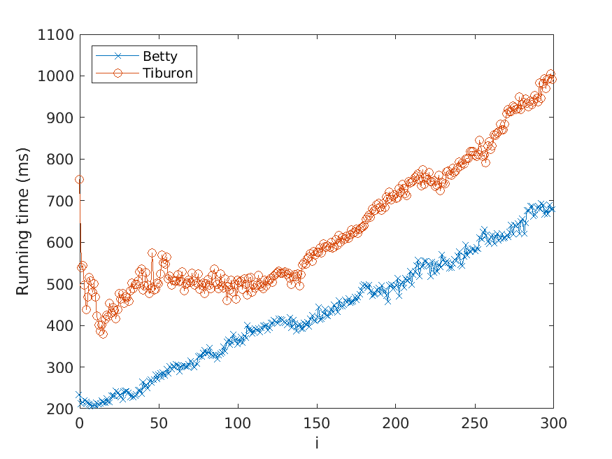
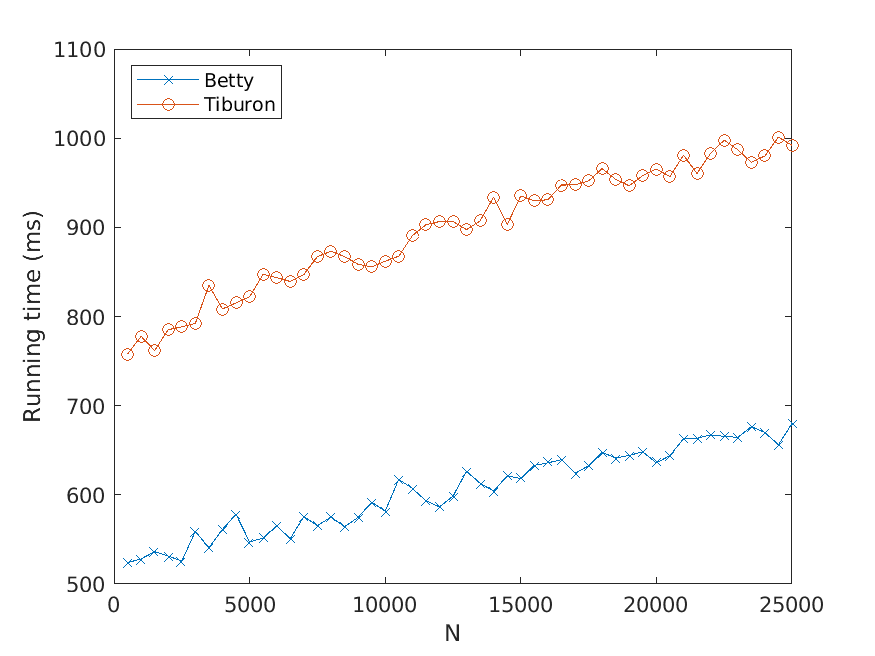
to expose the algorithms to challenging instances. Our results show that BETTY is gener-
ally more time efﬁcient than TIBURON, despite the fact that the former is more general
as it can also compute best trees (with almost the same efﬁciency as it computes best
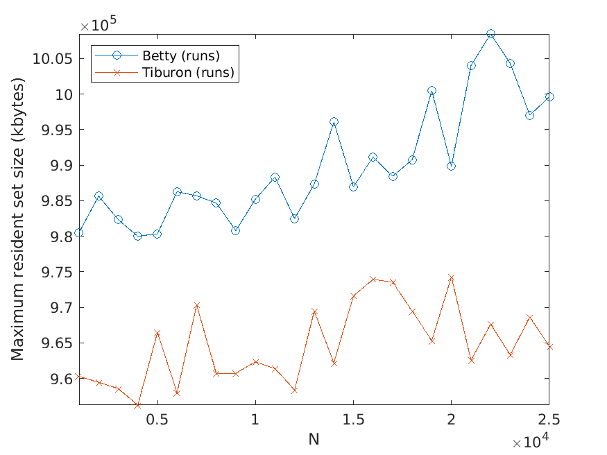
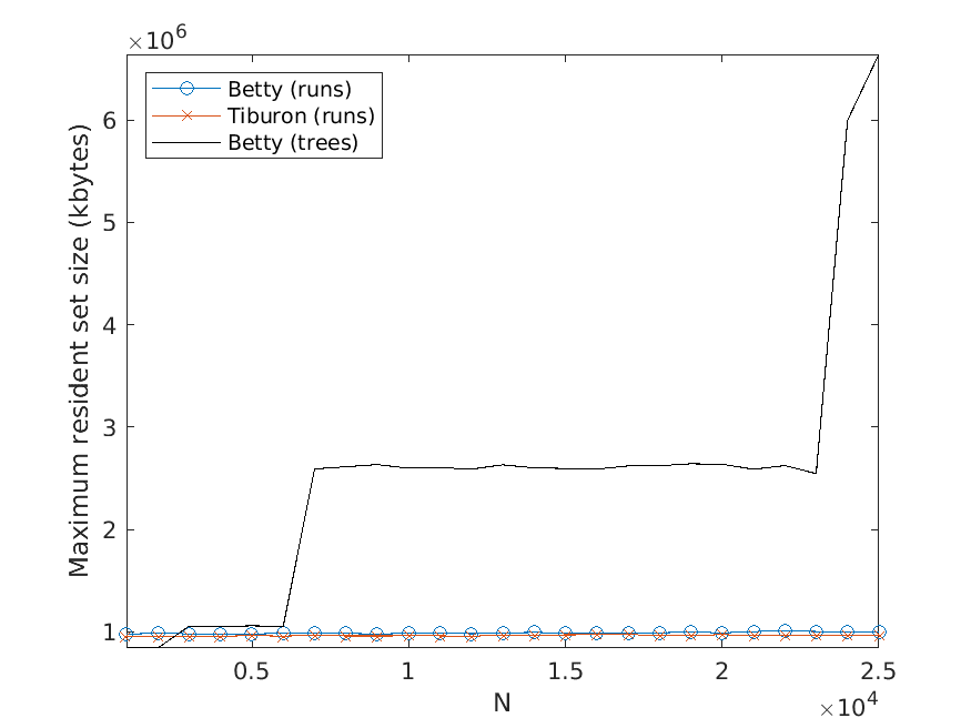
runs). Moreover, we perform a limited set of experiments measuring the memory usage
of the applications, and can conclude that overall, the memory efﬁciency of TIBURON is
slightly better than that of BEST TREES.

1.1 Related Work

The proposed algorithm adds to a line of research that spans two decades. It originates
with an algorithm by Eppstein (1998) that ﬁnds the N best paths from one source
node to the remaining nodes in a weighted directed graph. When applied to graphs
representing weighted string automata, the list returned by Eppstein’s algorithm may
in case of nondeterminism contain several paths that carry the same string, that is, the
list is not guaranteed to be free from duplicate strings. Four years later, Mohri and
Riley (2002) presented an algorithm that computes the N best strings with respect to
a weighted string automaton and thereby creates duplicate-free lists. To reduce the
amount of redundant computation, consisting in the exploration of alternative runs
on one and the same substring, they incorporate the N shortest paths algorithm by
Dijkstra (1959). Moreover, Mohri and Riley work with on-the-ﬂy determinization of the
input automaton M, which avoids the problem that the determinized automaton can

121

D
o
w
n
o
a
d
e
d

f
r
o
m
h

t
t

:
/
/

d
i
r
e
c
t
.

i
t
.

e
d
u
/
c
o

l
i
/

a
r
t
i
c
e
–
p
d

f
/

4
8
1
1
1
9
2
0
0
6
6
5
2
/
c
o

l
i

_
a
_
0
0
4
2
7
p
d

b
y
g
u
e
s
t

o
n
0
7
S
e
p
e
m
b
e
r
2
0
2
3

Computational Linguistics

Volume 48, Number 1

be exponentially larger than M, but has at most one run on each input string. Jim´enez
and Marzal (2000) lift the problem to the tree domain by ﬁnding the N best parse trees
with respect to a context-free grammar in Chomsky normal form for a given string.
Independently, Huang and Chiang (2005) published an algorithm that computes the
best runs for weighted hypergraphs (which is equivalent to weighted tree automata
and weighted regular tree grammars), and that is a generalization of the algorithm by
Jim´enez and Marzal in that it does not require the input to be in normal form. Huang
and Chiang combine dynamic programming and lazy evaluation to keep the number of
intermediate computations small, and derive a lower bound on the worst-case running
time of their algorithm than Jim´enez and Marzal do.

As previously mentioned, the algorithm by Huang and Chiang (2005) is imple-
mented in the Tiburon toolkit by May and Knight (2006). Its initial usage was as part
of a machine-translation pipeline, to extract the N best trees from a weighted tree
automaton. In connection with this work, Knight and Graehl (2005) noted that there
was no known efﬁcient algorithm to solve this problem directly. As an alternative
way forward, Knight and Graehl thus enumerate the best runs and discard duplicate
trees, until sufﬁciently many unique trees have been found. Since TIBURON is highly
optimized and the current state-of-the-art tool for best runs extraction, it is a natural
choice of reference implementation for an empirical evaluation of our solution. The
algorithm by Huang and Chiang (2005) was later generalized by B ¨uchse et al. (2010) to
allow a linear pre-order on the weights, as opposed to a total order. B ¨uchse et al. (2010)
also prove that the algorithm is correct on cyclic input hypergraphs, provided that the
Viterbi algorithm for ﬁnding an optimal run (Jurafsky and Martin 2009) is replaced by
Knuth’s algorithm (Knuth 1974).1

Also, Finkel, Manning, and Ng (2006) remark on the lack of sub-exponential algo-
rithms for the best trees problem. They propose an algorithm that approximates the
solution when the automaton is expressed as a cascade of probabilistic tree transducers.
The authors model the cascade as a Bayesian network and consider every step as a
variable. This allows them to sample a set of alternative labels from each prior step, to
propagate onward in the current step. The approximation algorithm runs in polynomial
time in the size of the input device and the number of samples, but the convergence rate
to the exact solution is not analyzed. To explain why their approach is preferable to
ﬁnding N best runs, they extract the N = 50 best runs from the Stanford parser and
observe that about half of the output trees are actually duplicates—enough to affect the
outcome of the processing pipeline. Thus, they argue, extracting the highest ranking
trees rather than the highest ranking runs is not only theoretically better, but is also of
practical signiﬁcance.

Finally, we note that the best trees problem also has applications outside of NLP.
In fact, whenever we are considering a set of objects, each of which can be expressed
uniquely by an expression in some particular algebra, and the set of expressions is
the language of a wta, then the best trees algorithm can be used to produce the best
objects. For instance, Bj ¨orklund, Drewes, and Ericson (2016) propose a restricted class
of hypergraphs that are uniquely described by expressions in a certain graph algebra, so
the best trees algorithm makes it possible to ﬁnd the optimal such graphs with respect
to a wta. The reason why the representation needs to be unique is that otherwise we
will have to check equivalence between objects as an added step. In the case of graphs,

1 This replacement had already been done in TIBURON, without an explicit remark.

122

D
o
w
n
o
a
d
e
d

f
r
o
m
h

t
t

:
/
/

d
i
r
e
c
t
.

i
t
.

e
d
u
/
c
o

l
i
/

a
r
t
i
c
e
–
p
d

f
/

4
8
1
1
1
9
2
0
0
6
6
5
2
/
c
o

l
i

_
a
_
0
0
4
2
7
p
d

b
y
g
u
e
s
t

o
n
0
7
S
e
p
e
m
b
e
r
2
0
2
3

Bj ¨orklund, Drewes, and Jonsson

Improved N-Best Extraction

this would mean deciding graph isomorphism, which is not known to be tractable in
general.

2. Preliminaries

We write N for the set of nonnegative integers, N+ for N \ {0}, and R+ for the set of
non-negative reals; N∞ and R∞
+ denote N ∪ {∞} and R+ ∪ {∞}, respectively. For n ∈ N,
[n] = {i ∈ N | 1 ≤ i ≤ n}. Thus, in particular, [0] = ∅ and [∞] = N. The cardinality of a
(countable) set S is written |S|. The n-fold Cartesian product of a set S with itself is
denoted by Sn.

The set of all ﬁnite sequences over S is denoted by S∗, and the empty sequence by
λ. A sequence of l copies of a symbol s is denoted by sl. Given a sequence σ = s1 · · · sn
of n elements si ∈ S, we denote its length n by |σ|. Given an integer i ∈ [n], we write σi
for the i-th element si of σ. For notational simplicity, we occasionally use sequences as if
they were sets, for example, writing s ∈ σ to express that s occurs in σ, or S \ σ to denote
the set of all elements of a set S that do not occur in the sequence σ.

A (commutative) semiring is a structure (D, ⊕, ⊗, 0, 1) such that both (D, ⊕, 0) and
(D, ⊗, 1) are commutative monoids, the semiring multiplication ⊗ distributes over the
semiring addition ⊕ from both left and right, and 0 is an annihilator for ⊗, that is,
0 ⊗ d = 0 = d ⊗ 0 for all d ∈ D. In this article, we will exclusively consider the tropical
semiring. Its domain is R∞
+ , with min serving as semiring addition and ordinary plus as
semiring multiplication.

For a set A, an A-labeled tree is a partial function t : N∗

+ → A whose domain dom(t)
is a ﬁnite non-empty set that is closed to the left and under taking preﬁxes; whenever
+ and i ∈ N+, it holds that vj ∈ dom(t) for all 1 ≤ j ≤ i
vi ∈ dom(t) for some v ∈ N∗
(closedness to the left) and v ∈ dom(t) (preﬁx-closedness). The size of t is |t| = |dom(t)|.
An element v of dom(t) is called a node of t, and |{i ∈ N+ | vi ∈ dom(t)}| is the rank
of v. The subtree of t ∈ TΣ rooted at v is the tree t/v deﬁned by

dom(t/v) = {u ∈ N∗

+ | vu ∈ dom(t)}

and t/v(u) = t(vu) for every u ∈ N∗
rank of λ in t, then we denote t by f [t1, . . . , tk], which may be simpliﬁed to f if k = 0.

+. If t(λ) = f and t/i = ti for all i ∈ [k], where k is the

A ranked alphabet is a disjoint union of ﬁnite sets of symbols, Σ = (cid:83)

k∈N Σ(k). For
f ∈ Σ, the k ∈ N such that f ∈ Σ(k) is the rank of f , denoted by rank(f ). The set TΣ of
ranked trees over Σ consists of all Σ-labeled trees t in which the rank of every node
v ∈ dom(t) equals the rank of t(v). For a set T of trees we denote by Σ(T) the set of
trees which have a symbol from Σ at their root, with direct subtrees in T, more precisely,
{f [t1, . . . , tk] | k ∈ N, f ∈ Σ(k), and t1, . . . , tk ∈ T}.

In the following, let (cid:3) (cid:54)∈ Σ be a special symbol of rank 0. The set of contexts over Σ
is the set CΣ of trees c ∈ TΣ∪{(cid:3)} containing exactly one node v ∈ dom(c) with c(v) = (cid:3).
We deﬁne the depth of c to be depth(c) = |v|, i.e., the depth of c is the distance of (cid:3) from
the root of c. The substitution of another tree t into c results in the tree c[[t]] given by
dom(c[[t]]) = dom c ∪ {vu | u ∈ dom(t)} and, for all w ∈ dom (c[[t]]),

c[[t]](w) =

(cid:26)c(w) if w ∈ dom (c) \ {v}

t(u)

if w = vu for some u ∈ dom(t).

123

D
o
w
n
o
a
d
e
d

f
r
o
m
h

t
t

:
/
/

d
i
r
e
c
t
.

i
t
.

e
d
u
/
c
o

l
i
/

a
r
t
i
c
e
–
p
d

f
/

4
8
1
1
1
9
2
0
0
6
6
5
2
/
c
o

l
i

_
a
_
0
0
4
2
7
p
d

b
y
g
u
e
s
t

o
n
0
7
S
e
p
e
m
b
e
r
2
0
2
3

Computational Linguistics

Volume 48, Number 1

A weighted tree language over the tropical semiring is a mapping L : TΣ → R∞
+ ,
where Σ is a ranked alphabet. Weighted tree languages can be speciﬁed in a number of
equivalent ways. Three of the standard ones, mirroring the ways in which regular string
languages are traditionally speciﬁed, are weighted regular tree grammars, weighted
tree automata, and weighted ﬁnite-state diagrams formalized as hypergraphs. The
equivalence of the second and the third is shown explicitly in Jonsson (2021). All three
have been used in the context of N-best problems: weighted regular tree grammars by
May and Knight (2006), weighted tree automata by Bj ¨orklund, Drewes, and Zechner
(2019), and hypergraphs by Huang and Chiang (2005) and B ¨uchse et al. (2010). In this
article, we use weighted tree automata.

Deﬁnition 1
A weighted tree automaton (wta) over the tropical semiring is a system M = (Q, Σ, R,
ω, qf) consisting of:

•

a ﬁnite set Q of symbols of rank 0 called states;

a ranked alphabet Σ of input symbols disjoint with Q;
a ﬁnite set R ⊆ (cid:83)
k∈N Qk × Σ(k) × Q of transition rules;
a mapping ω : R → R+; and
a ﬁnal state qf ∈ Q.

w→ q to denote that τ = (q1, . . . , qk, f, q) ∈ R and
From here on, we write f [q1, . . . , qk]
ω(τ) = w, and consider R to be the set of these weighted rules, thus dropping the
component ω from the deﬁnition of M.

A transition rule τ : f [q1, . . . , qk]

w→ q will also be viewed as a symbol of rank k,
turning R into a ranked alphabet. We let tar(τ) denote the target state q of τ, src(τ)
denotes the sequence of source states q1 . . . qk, and rank (τ) = rank( f ). In addition, we
view every state q ∈ Q as a symbol of rank 0.

Deﬁnition 2
We deﬁne the set runsM ⊆ TR∪Q of runs ρ of M, their input trees inputM(ρ), their intrinsic
weights wtM(ρ), and their target state tar(ρ) inductively, as follows:

For every q ∈ Q, we have that q ∈ runsM with inputM(q) = q, wtM(q) = 0,
and tar(q) = q.

w→ q in R and all runs
For every transition rule τ : f [q1, . . . , qk]
ρ1, . . . , ρk ∈ runsM such that tar(ρi) = qi for all i ∈ [k], we let
ρ = τ[ρ1, . . . , ρk] ∈ runsM with

inputM(ρ) = f [inputM(ρ1), . . . , inputM(ρk)]

wtM(ρ) = w + (cid:80)
tar(ρ) = q

i∈[k] wtM(ρi) , and

124

D
o
w
n
o
a
d
e
d

f
r
o
m
h

t
t

:
/
/

d
i
r
e
c
t
.

i
t
.

e
d
u
/
c
o

l
i
/

a
r
t
i
c
e
–
p
d

f
/

4
8
1
1
1
9
2
0
0
6
6
5
2
/
c
o

l
i

_
a
_
0
0
4
2
7
p
d

b
y
g
u
e
s
t

o
n
0
7
S
e
p
e
m
b
e
r
2
0
2
3

Bj ¨orklund, Drewes, and Jonsson

Improved N-Best Extraction

The weight of a run ρ ∈ runsM is

M(ρ) =

(cid:26) wtM(ρ) if tar(ρ) = qf
otherwise.

∞

Now, the weighted tree language M : TΣ → R∞

+ recognized by M is given by

M(t) = min{M(ρ) | ρ ∈ runsM and inputM(ρ) = t}

for all t ∈ TΣ (where, by convention, min ∅ = ∞). In other words, M(t) is the minimal
weight of any run resulting in t – which is the sum of all weights of t in the tropical
semiring. Note that we, by a slight abuse of notation, denote by M both the wta and the
weight assignments to runs and trees it computes. Moreover, for q ∈ Q we deﬁne the
mapping Mq : CΣ → R∞
+ by Mq(c) = M(c[[q]]) for every c ∈ CΣ.

Throughout the rest of the article, we will generally drop the subscript M in runsM,

inputM, and wtM, because the wta in question will always be clear from the context.

Given as input a wta M and an integer N ∈ N, the N-best runs problem consists in
computing a sequence of N runs of minimal weight according to M. More precisely, an
algorithm solving the problem will output a sequence ρ1, ρ2, . . . of N pairwise distinct
runs such that there do not exist i ∈ [N] and ρ ∈ runs \ {ρ1, . . . , ρi} with M(ρ) < M(ρi). General Assumption. To make sure that the N-best runs problem always possesses a solution, and to simplify the presentation of our algorithms, we assume from now on that all considered wtas M have inﬁnitely many runs ρ such that tar(ρ) = qf. In particular, TΣ is assumed to be inﬁnite. Apart from simplifying some technical details, this assumption does not affect any of the reasonings in the paper. Similarly to the N-best runs problem, the N-best trees problem for the wta M consists in computing a sequence of pairwise distinct trees t1, t2, . . . in TΣ of minimal weight. In other words, we seek a sequence of trees such that there do not exist i ∈ [N] and t ∈ TΣ \ {t1, . . . , ti} with M(t) < M(ti). Note that the N-best trees problem always has a solution because we assume that TΣ is inﬁnite. Example 1 Figure 1 shows an example wta, and Table 1 contains a side-by-side comparison of the input trees of the 10 best runs and the 10 best trees of the automaton. Because the weight of every transition rules is 1, the weight of every run on an input tree t is its size |t|. Looking at the rules, we obtain the following recursive equations for the number #i(t) of runs ρ on a tree t ending in state tar(ρ) = qi: #0(a) = 1 #1(a) = 1 #0( f [t0, t1]) = #0(t0)#1(t1) + #1(t0)#0(t1) + #1(t0)#1(t1) #1( f [t0, t1]) = #0(t0)#0(t1) Hence, every tree t will occur #0(t) times in an N-best list based on best runs (provided that N is large enough). 125 l D o w n o a d e d f r o m h t t p : / / d i r e c t . m i t . e d u / c o l i / l a r t i c e - p d f / / / / 4 8 1 1 1 9 2 0 0 6 6 5 2 / c o l i _ a _ 0 0 4 2 7 p d . f b y g u e s t t o n 0 7 S e p e m b e r 2 0 2 3 Computational Linguistics Volume 48, Number 1 f f a q1 f q0 f a 1→ qi for i ∈ {0, 1} 1→ q1−i for i ∈ {0, 1} 1→ q0 for {i, j} = {0, 1} f [qi, qi] f [qi, qj] Figure 1 A ﬁnite-state diagram representing an example wta. The input alphabet is Σ(0) ∪ Σ(2), where Σ(0) = {a} and Σ(2) = {f }. Circles represent states (double circles indicate the ﬁnal state, i.e., qf = q0), and squares represent transitions (all of weight 1). The consumed input symbols are shown inside the squares. Undirected edges connect states in left-hand sides to consumed input symbols in counter-clockwise order, starting at noon. Directed arcs point from the consumed symbol to the right-hand side state of the transition in question. Table 1 The input trees of 10 best runs (left) in comparison with 10 best trees (right) for the wta in Figure 1. Best runs Best trees Input tree a f [a, a] f [a, a] f [a, a] f [a, f [a, a]] f [f [a, a], a] f [a, f [a, a]] f [f [a, a], a] f [a, f [a, a]] f [f [a, a], a] Weight 1 3 3 3 5 5 5 5 5 5 Tree a f [a, a] f [f [a, a], a] f [a, f [a, a]] f [f [a, a], f [a, a]] f [f [f [a, a], a], a] f [f [a, f [a, a]], a] f [a, f [f [a, a], a]] f [a, f [a, f [a, a]]] f [f [a, f [a, a]], f [a, a]] Weight 1 3 5 5 7 7 7 7 7 9 We end this section by discussing the choice of our particular weight structure, the tropical semiring. In the literature on wta, Deﬁnitions 1 and 2 are generalized to wta over arbitrary commutative semirings, and their resulting weighted tree lan- guages, simply by replacing + and min by ⊕ and ⊗, respectively. The tropical semiring (R∞ + , min, +, ∞, 0) used in Deﬁnitions 1 and 2 is frequently used in natural language processing. Equally popular is the Viterbi semiring ([0, 1], max, ·, 0, 1) that acts on the unit interval of probabilities, with maximum and standard multiplication as operations. In the setting discussed here, both semirings are equivalent. To see this, transform a wta M over the Viterbi semiring to a wta M(cid:48) over the tropical semiring by simply mapping every weight p of a transition rule of M to − ln p, that is, taking negative logarithms ev- erywhere. Since − ln p + − ln p(cid:48) = − ln(p · p(cid:48)) and − ln p < − ln p(cid:48) ⇐⇒ p > p(cid:48), it holds

126

D
o
w
n
o
a
d
e
d

f
r
o
m
h

t
t

:
/
/

d
i
r
e
c
t
.

i
t
.

e
d
u
/
c
o

l
i
/

a
r
t
i
c
e
–
p
d

f
/

4
8
1
1
1
9
2
0
0
6
6
5
2
/
c
o

l
i

_
a
_
0
0
4
2
7
p
d

b
y
g
u
e
s
t

o
n
0
7
S
e
p
e
m
b
e
r
2
0
2
3

Bj ¨orklund, Drewes, and Jonsson

Improved N-Best Extraction

that M(t) (now calculated using the Viterbi semiring operations) is equal to exp(−M(cid:48)(t))
for all trees t. It follows that the trees t1, . . . , tN form an N-best list according to M (now
looking for trees with maximal weights) if and only if they form an N-best list according
to M(cid:48) in the sense deﬁned above.

3. The Improved Best Trees Algorithm

In this section, we explain how the algorithm in Bj ¨orklund, Drewes, and Zechner (2019)
can be made lazier, and hence more efﬁcient, by exploring the search space with respect
to transitions rather than states. From here on, let M = (Q, Σ, R, qf) be a wta with m
transition rules, n states, and a maximum rank of r among the symbols in Σ.

3.1 BEST TREES V.1

We ﬁrst summarize the approach of Bj ¨orklund, Drewes, and Zechner (2019). The algo-
rithm maintains two data structures: an initially empty set T that collects all processed
trees, and a priority queue K of trees in Σ(T) that will be examined next. The priority of
a tree t in K is determined by the minimal value in the set of all M(c[[t]]), where c ranges
over all possible contexts. Let Mq denote the wta obtained from M by making q its ﬁnal
state. Then, for every context c and all trees t,

M(c[[t]]) = min
q∈Q

(Mq(c) + Mq(t))

(1)

Because Mq(c) is independent of t, it is possible to compute in advance a best context
cq that minimizes it. The technique will be discussed in Section 3.2.

Deﬁnition 3
A best context of a state q ∈ Q is a context cq with

Mq(cq) = min
c∈CΣ

Mq(c).

The value Mq(cq) is denoted by wq.

The algorithm uses the best contexts to compute an optimal state opt(t) for each tree
t that it encounters: opt(t) = argminq∈Qcq[[t]]. Throughout the article, we shall make use
of the following weight functions derived from M, where t ∈ TΣ:

∆q(t) = wq + Mq(t)

∆(t) = M(copt(t)[[t]])

D
o
w
n
o
a
d
e
d

f
r
o
m
h

t
t

:
/
/

d
i
r
e
c
t
.

i
t
.

e
d
u
/
c
o

l
i
/

a
r
t
i
c
e
–
p
d

f
/

4
8
1
1
1
9
2
0
0
6
6
5
2
/
c
o

l
i

_
a
_
0
0
4
2
7
p
d

b
y
g
u
e
s
t

o
n
0
7
S
e
p
e
m
b
e
r
2
0
2
3

Note that ∆(t) = minc∈CΣ M(c[[t]]) = minq∈Q ∆q(t).

The priority queue K is initialized with the trees in Σ0. Its priority order 0).

(cid:96)) with j(cid:48)

1, . . . , j(cid:48)

Note that j(cid:48)

i ≤ ji for all i ∈ [(cid:96)] implies that ∆qv (u(cid:48)(cid:48)) ≤ ∆qv (u(cid:48)) since Tp1, . . . , Tp(cid:96) are ap-
propriate. Hence, the inequality ∆τ(cid:48) (u(cid:48)(cid:48)) ≤ ∆τ(cid:48) (u(cid:48)) < ∆τ(u) contradicts the assumption that u was dequeued on line 13. We have thus proved (2). Because τ[u] is appended to Tq on line 15, it remains to be shown that Mq(τ[w]) ≤ Mq(τ[u]) for all trees τ[w] that have been appended to Tq during earlier iterations. Choosing q as q(cid:48), τ[u] as t, and w as u in (2) we get Mq(τ[u]) = ∆q(τ[u]) − wq ≥ ∆τ(w) − wq ≥ ∆q(τ[w]) − wq = Mq(τ[w]) where the ﬁrst inequality holds by the appropriateness of Tq and the second holds because tar(τ) = q. Furthermore, by (2) there is no tree t(cid:48) ∈ TΣ \ Tq such that Mq(t(cid:48)) < Mq(τ[u]). Thus, Tq is still appropriate when τ[u] has been appended to it. Lemma 2 Algorithm 2(cid:48) computes a solution to the N-best trees problem. 133 l D o w n o a d e d f r o m h t t p : / / d i r e c t . m i t . e d u / c o l i / l a r t i c e - p d f / / / / 4 8 1 1 1 9 2 0 0 6 6 5 2 / c o l i _ a _ 0 0 4 2 7 p d . f b y g u e s t t o n 0 7 S e p e m b e r 2 0 2 3 Computational Linguistics Volume 48, Number 1 Proof. We ﬁrst observe that, due to the output condition on line 17 of Algorithm 2(cid:48), the sequence of trees outputted by the algorithm does not contain repetitions. Next, whenever a tree s = τ[u] is outputted on line 18, we show that M(t) ≥ M(s) w→ q. Then q = qf for all trees t ∈ TΣ that have not yet been outputted. Let τ : f [q1, . . . , qk] and thus cq = (cid:3), wq = 0, and M(s) = ∆τ(u). Now, consider any t ∈ TΣ that has not yet been outputted. Then we have t ∈ TΣ \ Tqf. Consequently, M(t) = ∆qf (t) ≥ ∆τ(u) by Lemma 1, as required. To complete the proof, we have to show that there cannot be an inﬁnite number of iterations without any tree being outputted. We show the following, stronger statement: Claim 1. Let δ = maxq∈Q δq, where δq is deﬁned as in Equation 2 for all q ∈ Q. At any point in time during the execution of Algorithm 2(cid:48), it takes at most δ iterations until the selected transition rule τ satisﬁes tar(τ) = qf. To see this, let Kτ be dequeued on line 12 and let q = tar(τ). If q = qf, the statement holds. Otherwise, the context cq has the form cq(cid:48) [[g[tbest p1 , . . . , tbest pi−1, (cid:3), tbest pi+1, . . . , tbest p(cid:96) ]]] for a transition rule τ(cid:48) : g[p1, . . . , p(cid:96)] Tq, say at position n. It follows that t(cid:48) = τ(cid:48)[u(cid:48)] with w(cid:48) → q(cid:48) with pi = q. The tree t = τ[u] is appended to u(cid:48) = (1, . . . , 1 (cid:124) (cid:123)(cid:122) (cid:125) i−1 , n, 1, . . . , 1 (cid:124) (cid:123)(cid:122) (cid:125) (cid:96)−i−1 ) becomes deﬁned, where t(cid:48) = g[tbest p1 , . . . , tbest pi−1, t, tbest pi+1, . . . , tbest p(cid:96) ]. We also know that l D o w n o a d e d f r o m h t t p : / / d i r e c t . m i t . e d u / c o l i / l a r t i c e - p d f / / / / 4 8 1 1 1 9 2 0 0 6 6 5 2 / c o l i _ a _ 0 0 4 2 7 p d . f b y g u e s t t o n 0 7 S e p e m b e r 2 0 2 3 1. 2. 3. there is no u(cid:48)(cid:48) in any of the queues Kτ(cid:48)(cid:48) with ∆τ(cid:48)(cid:48) (u(cid:48)(cid:48)) < ∆τ(u) (Lemma 1(2)), ∆τ(cid:48) (u(cid:48)) = M(cq[[t]]) = M(cq(cid:48) [[t(cid:48)]]) = ∆τ(u), and δq(cid:48) = δq − 1. It follows that the queue Kτ(cid:48)(cid:48) from which a tuple is dequeued on line 12 at the start of the next iteration satisﬁes δtar(τ(cid:48)(cid:48) ) = δq − 1, thus bounding the number of iterations until this quantity reaches 0 from above by δ. Now, to ﬁnish the proof, note that τ[u] (cid:54)= τ[u(cid:48)] whenever u (cid:54)= u(cid:48) because the se- quences Tq, q ∈ Q, do not contain repetitions. Because, furthermore, no tuple u is en- queued twice in Kτ, line 18 will be reached after at most δ iterations. We ﬁnally show that Algorithm 2 is correct as well. Theorem 1 Algorithm 2 computes a solution to the N-best trees problem. Proof. Consider an execution of Algorithm 2(cid:48) and assume that we assign every tree a color, red or black, where black is the default color. (The color attribute of a subtree may differ from that of the tree itself.) Suppose that, in an iteration of the main loop, we have w→ q and u = (i1, . . . , ik), and thus τ[u] = f (t1, . . . , tk) where tj = (Tqj )ij for τ : f [q1, . . . , qk] 134 Bj ¨orklund, Drewes, and Jonsson Improved N-Best Extraction all j ∈ [k]. If |Tq| ≥ N on line 14 and we append τ[u] to it on line 15, we color τ[u] red while its subtrees t1, . . . , tk keep their colors as given by their positions in Tq1, . . . , Tqk . Now, assume that some Tq contains a tree t = f [t1, . . . , tk] such that tj is red for some j ∈ [k]. We show that this implies that t is red. We know that t was appended to Tq as a tree of the form τ[u] for some u = (i1, . . . , ik) with ij > N (because of the assumption that
tj is red). We know also that earlier iterations have dequeued all tuples from Kτ of the
form ui = (i1, . . . , ij−1, i, ij+1, . . . , ik) for i = 1, . . . , N. (This is an immediate consequence
of Lemma 2 because, by Lemma 1(1), ∆τ(ui) < ∆τ(u) for all i ∈ [k].) Since the τ[ui] are pairwise distinct (as they differ in the j-th direct subtree) this means that |Tq| ≥ N before τ[u] was enqueued, thus proving that t is red, as claimed. Because Algorithm 2(cid:48) terminates when |Tqf | = N, none of the trees in Tqf will ever be red. By the above, this implies that all subtrees of trees in Tqf are black as well. As subtrees inherit their color from the Tq they are taken from, this shows that no red tree occurring in an execution of Algorithm 2(cid:48) can ever have an effect on the output of the algorithm. Hence, the output of Algorithm 2 is the same as that of Algorithm 2(cid:48) and the (cid:3) result follows from Lemma 2. 3.5 Time Complexity Recall that the input M = (Q, Σ, R, qf) is assumed to be a wta with m transition rules, n states, and a maximum rank of r among its symbols. In the complexity analysis, we consider an efﬁcient implementation of Algorithm 2 along the lines illustrated in Figure 2, with priority queues based on heaps (Cormen et al. 2009). This enables us to implement the following details efﬁciently: • • w→ q. At a given stage of the algorithm, Consider a transition τ : f [q1, . . . , qk] some of the elements u = (u1, . . . , uk) in Kτ may contain elements ui such | < ui, that is, τ[u] is still undeﬁned and hence ∆τ(u) = ∞. Thus, that |Tqi ∆τ(u) must be decreased from ∞ to its ﬁnal value in R∞ | has + when |Tqi reached ui for all i ∈ [k]. For this, we record for every p ∈ Q and for |Tp| < j < |N| a list of all u ∈ Kτ such that τ is as above, qi = p for some i ∈ [k], and ui = j. When |Tp| reaches the value j, this list is used to adjust the priority of each u on that list to the new value of ∆τ(u) (which is either still ∞ or has reached its ﬁnal value). The queue K(cid:48) that contains the individual queues Kτ as elements is implemented in the straightforward way, also using priority queues based on heaps. As described earlier, the priority between Kτ and Kτ(cid:48) is given by comparing their top-priority elements: if these elements are u and u(cid:48), respectively, then Kτ takes priority over Kτ(cid:48) if (∆τ(u), δtar(τ)) < (∆τ(cid:48) (u(cid:48)), δtar(τ(cid:48) )). If one of the queues Kτ runs empty (which can only happen if rank(τ) = 0), then Kτ is removed from K. We now establish an upper bound on the running time of the algorithm. Theorem 2 Algorithm 2 runs in time O(Nm(log(m) + r2 + r log(Nr))) 135 l D o w n o a d e d f r o m h t t p : / / d i r e c t . m i t . e d u / c o l i / l a r t i c e - p d f / / / / 4 8 1 1 1 9 2 0 0 6 6 5 2 / c o l i _ a _ 0 0 4 2 7 p d . f b y g u e s t t o n 0 7 S e p e m b e r 2 0 2 3 Computational Linguistics Volume 48, Number 1 Proof. For the proof, we look at the maximum number of instantiations that we en- counter during a run of the algorithm. Because K(cid:48) contains (at most) the m queues Kτ, enqueuing into K(cid:48) is in O(log(m)). Furthermore, each rule is limited to N instantiations, due to the fact that the sequences Tq do not contain repetitions and thus τ[u] (cid:54)= τ[u(cid:48)] for u (cid:54)= u(cid:48). This implies that the maximum number of iterations of the main loop is Nm, yielding an upper bound of O(Nm log(m)) for the management of K(cid:48). Next, we have the rule-speciﬁc queues Kτ. Each time a tuple u ∈ Nk is dequeued from Kτ, at most |inc(u)| = k ≤ r new tuples are enqueued. In total, the creation of these k tuples of size k each takes k2 ≤ r2 operations. Thus, there will be at most Nr elements in Kτ for any τ, which gives us a time bound of O(log(Nr)) per queue operation, a total time of O(N(r2 + r log(Nr))) for the management of Kτ, and thus a total of O(Nm(r2 + r log(Nr))) for the m queues Kτ altogether. Summing up the upper bounds for the management of the two queue types yields O (cid:0)Nm(log(m) + r2 + r log(Nr))(cid:1) as claimed. To complete the analysis, we have to argue that the time that needs to be spent to check whether τ[u] has been outputted before, can be made negligible. We do this by implementing the forest of outputted trees in such a way that equal subtrees are shared. Hence, trees are equal if (and only if) they have the same address in memory. Assuming a good hashing function, the construction of τ[u] from the (already previ- ously constructed) trees referred to by u, can essentially be done in constant time. Now, if we maintain with every previously constructed tree a ﬂag (cid:88) indicating whether that tree had already been outputted once, the test boils down to constructing τ[u] (which (cid:3) would return the already existing tree if it did exist) and checking the ﬂag (cid:88). The running time of Algorithm 2 should be contrasted with the running time O (cid:0)max(Nmn · (Nr + r log r + N log N), N2n3, mr2)(cid:1) of Algorithm 1 (Bj ¨orklund, Drewes, and Zechner 2019). By handling instantiations of transition rules rather than states, we reduce the running times of the algorithm roughly by a factor of O(Nn). We have not performed a detailed space complexity analysis, but because we know that the logarithmic factors are due to heap operations, we can conclude that the memory space consumption of the algorithm is in O(Nm). In practical applications, we expect to see Algorithm 2 used in two ways. The ﬁrst is, as discussed in the Introduction, the situation in which N best trees are computed for a relatively small value of N, for example, N = 200 as suggested by Socher et al. (2013). Here, based on a comparison of the upper bounds on the running time, and assuming that they are reasonably tight, Algorithm 2 will outperform Algorithm 1 if m, which we believe is the common case. In the second scenario, N is larger than Algorithm 2 is invoked with a very large N to enumerate the trees recognized by the input automaton, outputting them in ascending order by weight. In this scenario, our exploration by transition rule is even more valuable, as it saves redundant computation. √ 136 l D o w n o a d e d f r o m h t t p : / / d i r e c t . m i t . e d u / c o l i / l a r t i c e - p d f / / / / 4 8 1 1 1 9 2 0 0 6 6 5 2 / c o l i _ a _ 0 0 4 2 7 p d . f b y g u e s t t o n 0 7 S e p e m b e r 2 0 2 3 Bj ¨orklund, Drewes, and Jonsson Improved N-Best Extraction 4. The Algorithm BEST RUNS We now recall the algorithm by Huang and Chiang (2005), which we henceforth will refer to as BEST RUNS. To facilitate comparison, we express BEST RUNS in terms of wta. The type of wta used as input to BEST RUNS differs slightly from the one used in Deﬁnition 1 in that the admissible weight structures are not restricted to the tropical semiring. Instead, each transition rule τ : f [q1, . . . , qk] → q is equipped with a weight + → R+. The deﬁnition of the weight of a run ρ = τ[ρ1, . . . , ρk] is then function wtτ : Rk changed to wt(ρ) = wtτ(wt(ρ1), . . . , wt(ρk)). For the algorithm to work, these weight functions wtτ are required to be monotonic: wtτ(w1, . . . , wk) ≥ wtτ(w(cid:48) k) whenever wi ≥ w(cid:48) i for all i ∈ [k]. Deﬁnition 1, which BEST TREES is based on, corresponds to the special case where each of these weight functions is of the form wtτ(w1, . . . , wk) = w + (cid:80) i∈[k] wi for a constant w. In other words, the weight functions BEST TREES can work with are a restriction of those BEST RUNS works on. This will be discussed in Section 5. 1, . . . , w(cid:48) The input to BEST RUNS is a pair (M, N), where M is a wta with m transition rules and n states, and N ∈ N. The algorithm is outlined in Algorithm 3. Line 2 is a preprocessing step that can be performed in O(m) time using the Viterbi algorithm, given that the rank of the alphabet used is considered a constant. A list input[q] is used to store, for each state q ∈ Q, the at most N discovered best runs arriving at q. The search space of candidate runs is represented by an array of heaps, here denoted cands. For each state q, cands[q] holds a heap storing the (at most N) best, so far unexploited, runs arriving at q. That is, if we have already picked the N(cid:48) best runs arriving at a node, the heap lets us pick the next best unpicked candidate efﬁciently when so requested by the recursive call. To expand the search space, the N(cid:48)-th best run ρ is used as follows: if τ = ([q1, . . . , qk] → q), we obtain a new candidate by replacing the i-th direct subtree of ρ with the next (and thereby minimally worse) run in input arriving at qi. Note that this is equivalent to the increment method used in BEST TREES. As shown by Huang and Chiang (2005), the worst case running time of BEST RUNS is O(m log |V| + smaxN log N) where smax is the size of the largest run among the N results.4 Using similar reasoning for the memory complexity as for BEST TREES, BEST RUNS achieves a O(m + smaxN) memory complexity bound. 5. Comparison A major difference between BEST RUNS and BEST TREES is that the former solves the N-best runs problem whereas the latter solves the N-best trees problem: On lines 14 and 17 of Algorithm 2, duplicate trees are discarded. If these conditions are removed, BEST TREES solves the best runs problem. (Provided, of course, that the objects outputted are changed to being runs rather than trees.) For the sake of comparison, we adopt the view of Huang and Chiang (2005) that the ranked alphabet Σ can be considered ﬁxed. This yields that the running time of BEST TREES is O(Nm(log m + log N)). Since m ∈ O(nr+1), where r is the (now ﬁxed) maximal rank of symbols in Σ, it follows that log m ∈ O(log n), so the second expression 4 In fact, the running time obtained by Huang and Chiang (2005) is O(m + smaxN log N), but this assumes (the graph representation of) M to be acyclic. When M is cyclic, line 2 must be implemented by using Knuth’s algorithm, resulting in an additional factor log n in the ﬁrst term. 137 l D o w n o a d e d f r o m h t t p : / / d i r e c t . m i t . e d u / c o l i / l a r t i c e - p d f / / / / 4 8 1 1 1 9 2 0 0 6 6 5 2 / c o l i _ a _ 0 0 4 2 7 p d . f b y g u e s t t o n 0 7 S e p e m b e r 2 0 2 3 Computational Linguistics Volume 48, Number 1 simpliﬁes to Nm(log n + log N) ≤ m log n · N log N. Moreover, recall that the worst case running time of BEST RUNS is O(m log n + smaxN log N). If N is large enough to make the second term the dominating one, the difference between both running times is thus a factor of (m log n)/smax (assuming for the sake of the comparison that the given bounds are reasonably tight). A further comparison between the running times does not appear to be all that meaningful because smax depends on both N and the structure of the input wta, and the algorithms are specialized for different problems. q q return , . . . , ρbest if |input[q]| ≥ N then arriving at q, for every q ∈ Q end if if cands[q] is undeﬁned then tmp ← SORT-BY-WEIGHT({τ[ρbest qk q1 cands[q] ← HEAP-IFY(tmp[1] . . . tmp[N]) LIST-ADD(input[q], HEAP-EXTRACT-MIN(cands[q])) Algorithm 3 Compute N ∈ N∞ runs arriving at qf ∈ Q = [n] of minimal weight accord- ing to a wta M = (Q, Σ, R, qf) (Huang and Chiang 2005). 1: procedure BEST RUNS(M, N) Compute 1-best run ρbest 2: input[q] ← LIST-EMPTY() for all q ∈ Q 3: LIST-ADD(input[q], ρbest ) for all q ∈ V 4: BEST RUNS0(qf, N) 5: for ρ ∈ input[qf] do 6: output(ρ) 7: end for 8: 9: end procedure 10: 11: procedure BEST RUNS0(q, N) 12: 13: 14: 15: 16: 17: 18: 19: 20: 21: 22: 23: 24: 25: 26: end procedure 27: 28: procedure NEXT RUNS(qcands, ρ = τ[ρ1, . . . , ρk] where τ = ([q1, . . . , qk] → q)) 29: 30: 31: 32: 33: 34: 35: 36: 37: 38: 39: 40: 41: end procedure for i ← 1, . . . , k do list ← input[qi] N(cid:48) ← index of ρ in input[q] BEST RUNS0(qi, N(cid:48)) if N(cid:48) ≤ LIST-SIZE(list) then ρ(cid:48) i ← LIST-GET(list, N(cid:48)) ρ(cid:48) ← τ[ρ1, . . . , ρi−1, ρ(cid:48) if ρ(cid:48) /∈ qcands then s ← LIST-SIZE(input[q]) ρ ← LIST-GET(input[q], s) NEXT RUNS(cands[q], ρ) LIST-ADD(input[q], HEAP-EXTRACT-MIN(cands[q])) end if while LIST-SIZE(input[q]) < N and HEAP-SIZE(cands[q]) > 0 do

(cid:46) the s-best run arriving at q
(cid:46) build new candidates from ρ

(cid:46) make sure list has N(cid:48) ≤ N elements

] | τ = ([q1, . . . , qk] → q) ∈ R})

HEAP-INSERT(qcands, ρ(cid:48))

i, ρi+1, . . . , ρk]

end while

end for

end if

138

D
o
w
n
o
a
d
e
d

f
r
o
m
h

t
t

:
/
/

d
i
r
e
c
t
.

i
t
.

e
d
u
/
c
o

l
i
/

a
r
t
i
c
e
–
p
d

f
/

4
8
1
1
1
9
2
0
0
6
6
5
2
/
c
o

l
i

_
a
_
0
0
4
2
7
p
d

b
y
g
u
e
s
t

o
n
0
7
S
e
p
e
m
b
e
r
2
0
2
3

Bj ¨orklund, Drewes, and Jonsson

Improved N-Best Extraction

A conceptual comparison of the two algorithms may be more insightful. The al-
gorithms differ mainly in two ways. The ﬁrst difference is that, while BEST RUNS
enumerates candidates of best runs using one priority queue per node of G, BEST TREES
uses a more ﬁne-grained approach, maintaining one priority queue per hyperedge.
Since the upper bound on the length of queues is O(N) in both cases, in total BEST TREES
may need to handle O(Nm) candidates whereas BEST RUNS needs only O(Nn). This
ostensible disadvantage of BEST TREES is not a real one as it occurs only when solving
the N-best trees problem. The difference vanishes if the algorithm is used to compute
best runs (by changing lines 14 and 17). To see this, consider a given state q ∈ Q. Each
time a queue element (i1, . . . , ik) is dequeued from a queue Kτ with τ : f [q1, . . . , qk] → q,
the corresponding run is appended to the list Tq on line 15, and k queue elements are
inserted on line 21. As this can only happen at most N times per state q, in total only
O(Nn) queue elements are ever created in the worst case. In other words, if BEST TREES
is set to solve the N-best runs problem, the splitting of queues does not result in a
disadvantage compared to BEST RUNS.

The second conceptual difference between the algorithms is that BEST TREES adopts
an optimization technique known from the N-best strings algorithm by Mohri and Riley
(2002). It precomputes and uses (the weight and depth of) a best context cq for every state
q in order to explore the search space in a more goal-oriented fashion. The possibility
of using this optimization depends on the use of the tropical semiring. As mentioned
in the Introduction, B ¨uchse et al. (2010) extend the algorithm of Huang and Chiang
to structured weight domains. This does not seem to be possible for Algorithm 2 (nor
for Algorithm 1). The reason is that the computation and use of best contexts requires
that the semiring is extremal, which is the case for the tropical semiring, but not for
structured weight domains in general. Let (cid:96) be the maximum of the distances of states
in Q to qf, that is,

(cid:96) = max
q∈Q

dist(q, qf)

where dist(q, qf) denotes the length of the shortest sequence of transition rules τ0 · · · τn
such that q ∈ src(τ0), tar(τi−1) ∈ src(τi) for all i ∈ [n], and qf = tar(τn). The argument
used to show Claim 1 in the proof of Lemma 2 yields that, at every point in time at most
(cid:96) further loop executions are made before the next best run is outputted. To see this,
consider an execution of the main loop, in which a run ρ = τ[· · · ] arriving at a state q
is constructed. The priority of the corresponding queue element on line 13 is given by
(wt(ρ) + w, d), where w and d are the weight and depth of cq. If q (cid:54)= qf, then cq (cid:54)= (cid:3), and
thus it is of the form cq(cid:48) [[τ(cid:48)[ρ1, . . . , ρi−1, (cid:3), ρi+1, . . . , ρk]]], where the ρj are the 1-best runs
arriving at their respective nodes (see Figure 3).

It follows that line 21 inserts the element into Kτ that represents the run ρ(cid:48) =
τ(cid:48)[ρ1, . . . , ρi−1, ρ, ρi+1, . . . , ρk]. Because each of the runs ρi, arriving at some state qi,
is already in the respective list Tqi , the run ρ(cid:48) immediately becomes a current candi-
date arriving at q = tar(τ). The corresponding pair (wq, dq) = (wt(cq), depth(cq)) satisﬁes
wq + wt(ρ(cid:48)) = w + wt(ρ) and dq = d − 1. Hence, ρ(cid:48) (or another run with the same prior-
ity) will be picked in the next loop execution, meaning that after at most (cid:96) steps the node
arrived at by the constructed run will be qf, that is, the run will be outputted. This also
shows that queues the elements of which are not needed for generating output trees
will never become ﬁlled beyond their initial element.

We end the comparison by looking at Table 2, which summarizes the discussion
above and provides comparison data for the other N-best algorithms discussed in this

139

D
o
w
n
o
a
d
e
d

f
r
o
m
h

t
t

:
/
/

d
i
r
e
c
t
.

i
t
.

e
d
u
/
c
o

l
i
/

a
r
t
i
c
e
–
p
d

f
/

4
8
1
1
1
9
2
0
0
6
6
5
2
/
c
o

l
i

_
a
_
0
0
4
2
7
p
d

b
y
g
u
e
s
t

o
n
0
7
S
e
p
e
m
b
e
r
2
0
2
3

Computational Linguistics

Volume 48, Number 1

(cid:96)

best context cq

(cid:96) − 1

best context cp

τ(cid:48)

dequeued
run ρ

· · ·

ρ1

ρi−1

· · ·

ρi+1

ρk

dequeued
run ρ

· · ·

(cid:96) − 1

best context cp

τ(cid:48)

nextnext
dequeued run ρ(cid:48)
dequeued run ρ(cid:48)

· · ·

Figure 3
When a run ρ reaching state q is dequeued with (cid:96) > 0 (top left), then its best context cq is of the
form cp[[τ(cid:48)[ρ1, . . . , ρi−1, (cid:3), ρi+1, . . . , ρk]]], where cp is the best context for p = tar(τ(cid:48)) and the ρi are
1-best trees reaching the remaining states of τ(cid:48) (top right). Hence, ρ(cid:48) = τ(cid:48)[ρ1, . . . , ρi−1, ρ, ρi+1, . . . , ρk]
(or a run which likewise is less than (cid:96) steps away from an output run) will be the next run
dequeued (bottom).

article. Keep in mind that N must be interpreted differently depending on the problem
at hand. For example, the output of BEST RUNS is not equivalent to the output of BEST
TREES (unless the input is deterministic), which is why we cannot directly compare
the time complexities. This output inequivalence should also be considered in Section 7
where, for simplicity, we plot data for BEST RUNS and BEST TREES side by side.

140

D
o
w
n
o
a
d
e
d

f
r
o
m
h

t
t

:
/
/

d
i
r
e
c
t
.

i
t
.

e
d
u
/
c
o

l
i
/

a
r
t
i
c
e
–
p
d

f
/

4
8
1
1
1
9
2
0
0
6
6
5
2
/
c
o

l
i

_
a
_
0
0
4
2
7
p
d

b
y
g
u
e
s
t

o
n
0
7
S
e
p
e
m
b
e
r
2
0
2
3

Bj ¨orklund, Drewes, and Jonsson

Improved N-Best Extraction

Table 2
Summary of characteristics of N-best algorithms. For the time complexities, the alphabet is taken
to be constant and the input is represented as a wta. The two right-most columns indicate
whether the algorithms compute best contexts as a preprocessing step, and what optimization
methods are used to ﬁnd new candidate objects.

Algorithm

Objects

Time complexity

Best contexts

Eppstein (1998)

Paths

O(n log n + Nn + m)

Mohri and Riley (2002)

Strings

No formal analysis provided

Huang and Chiang
(2005)
BEST TREES V.1

BEST TREES

Runs

Trees

Trees
Runs

O(m log n + smaxN log N)5

O(N2n(n2 + m log N))

O(Nm(log m + log N))
O(N(log m + log N))6

Yes

Yes
Yes

Search-space
expansion
Adding sidetracks
to implicit heap
representations of
paths
On-the-ﬂy
determinization
Increment

Eppstein’s
algorithm
Increment
Increment

6. Implementation Details

In the upcoming section, we experimentally compare BEST RUNS and BEST TREES.
In preparation of that, we want to make a few comments on the implementation of
BEST TREES. As previously mentioned, BEST RUNS is implemented in the Java toolkit
TIBURON by May and Knight, and this is the implementation we use in our experiments.
Therefore, we simply refer to the TIBURON GitHub page7 for implementation details.

We have extended our code repository BETTY,8 which originally provided an im-
plementation of BEST TREES V.1, to additionally implement the improved BEST TREES
as its standard choice of algorithm. A ﬂag -runs can be passed on as an argument to
compute best runs instead of best trees. Below follow a number of central facts about
the BETTY implementation.

First, recall Algorithm 2, and in particular that the best tree tbest

is inserted into Tq
for all q ∈ Q prior to the start of the main loop rather than letting Tq be empty and
initializing Kτ to 1rank τ for all q ∈ Q and τ ∈ R. The reason is that the latter would not
guarantee that at most (cid:96) iterations are made until a run is outputted because some
ρi may still not be in Tq. If this happens, transition rules adding the weight 0 may
repeatedly be picked because some other τ(cid:48) is not yet enabled. However, with a trick
the initialization can nevertheless be simpliﬁed as indicated. The idea is to delay the
execution of line 22 for every queue Kτ until τ has actually appeared in an output tree.
Thus, until this has happened, Kτ is disabled from contributing another tree to Ttar(q).
This variant turned out to have efﬁciency advantages in practice and is therefore the
variant implemented in BETTY. Another advantage is that it allows BETTY to handle a set

5 Allows for cyclic input wta; smax is the size of the largest output.
6 Note that a factor m is removed, compared with when the same algorithm is used for ﬁnding the best

trees. This is because all runs originating at the same rule queue are distinct (and naturally the same also
holds for different rule queues).

7 https://github.com/isi-nlp/tiburon.
8 https://github.com/tm11ajn/betty.

141

D
o
w
n
o
a
d
e
d

f
r
o
m
h

t
t

:
/
/

d
i
r
e
c
t
.

i
t
.

e
d
u
/
c
o

l
i
/

a
r
t
i
c
e
–
p
d

f
/

4
8
1
1
1
9
2
0
0
6
6
5
2
/
c
o

l
i

_
a
_
0
0
4
2
7
p
d

b
y
g
u
e
s
t

o
n
0
7
S
e
p
e
m
b
e
r
2
0
2
3

Computational Linguistics

Volume 48, Number 1

of ﬁnal states rather than a single one. This is not possible with the original initialization
of Algorithm 2, because line 3 would have to be generalized to outputting the best
trees of all ﬁnal states, which cannot be done while maintaining the correctness of the
algorithm, since the second best tree for a state q may have a lesser weight than the best
tree for another state q(cid:48).

In lines 14 and 17 of Algorithm 2, trees are checked for equivalence. To perform
the comparisons efﬁciently, we make use of hash tables. We use immutable trees, which
need to be hashed only once when they are created; we then save the hash code together
with the tree to make the former accessible in constant time for each tree. To compare
trees for inequality, their hash codes are compared. If equal (which seldom happens if
the trees are not equal), the comparison is continued recursively on the direct subtrees.
This is theoretically less efﬁcient than the method of representing trees uniquely in
memory (as described in the last paragraph of the proof of Theorem 2), but practically
sufﬁcient and much easier to implement.

When creating new tuples for a transition rule τ as given by line 21, we add the
tuples that can be instantiated directly to the corresponding queue Kτ. The tuples
that cannot be instantiated must, however, be stored until they can. We want to be
able to efﬁciently access the tuples that are affected when adding a tree t to Tq(cid:48) for
some q(cid:48) ∈ Q (line 15). Therefore, we connect each tuple to the memory locations that
will contain the data needed by the tuple. In more detail: Let τ = ( f [q1 · · · qk] → q)
be any transition rule in R and let (i1, . . . , ik) be a tuple originating from τ. For every
ij ∈ {i1, . . . , ik}, the tuple is saved in a list of tuples affected by Tqj (ij) and marked with
a counter that shows how many trees remain until it can be instantiated. Thus, when
t is added to Tq(cid:48) (ij) for ij ∈ {i1, . . . , ik} and q(cid:48) = qj, we can immediately access all tuples
that can possibly be instantiated. If a tuple cannot be instantiated, its counter is de-
creased appropriately.

7. Experiments

Let us now describe our experiments. For each problem instance (i.e., combination of
input ﬁle and value of N), we perform a number of test runs, measure the elapsed time,
and compute the average over the test runs. To avoid noise in our data caused by, for
example, garbage collection, we only measure the time consumed by the thread the
actual application runs in. Also, we disregard the time it takes to read the input ﬁles.

The number of test runs that are performed per problem instance is decided by the
relationship between the mean µ and the standard deviation σ of the recorded times—
these values are computed every ﬁfth test run, and to ﬁnish the testing of the current
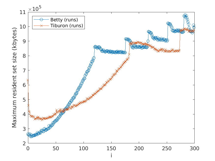
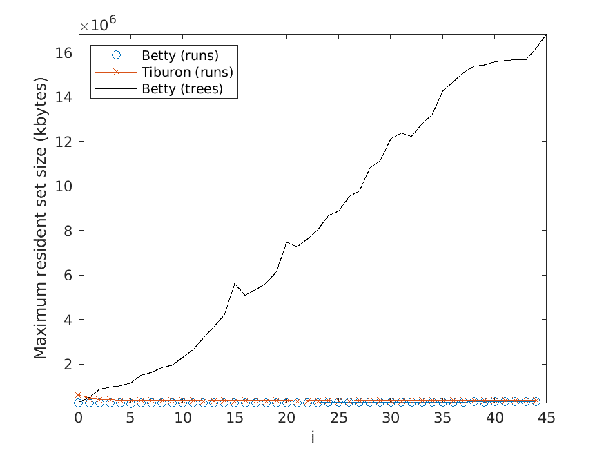
problem instance, we require that σ < 0.01µ. However, ﬁve test runs per problem instance has turned out to be sufﬁcient for fulﬁlling the requirement in practically all instances seen. The memory usage is measured in terms of the maximum resident set size of the application process by using the Linux time command. Moreover, the strategy described above for computing the average over several test runs is used here as well. All test scripts have been written in Python, in contrast to the tested implementa- tions, which use Java. We run the experiments on a computer with a 3.60 Hz Intel Core i7-4790 processor. 142 l D o w n o a d e d f r o m h t t p : / / d i r e c t . m i t . e d u / c o l i / l a r t i c e - p d f / / / / 4 8 1 1 1 9 2 0 0 6 6 5 2 / c o l i _ a _ 0 0 4 2 7 p d . f b y g u e s t t o n 0 7 S e p e m b e r 2 0 2 3 Bj ¨orklund, Drewes, and Jonsson Improved N-Best Extraction 7.1 Corpora The corpora that were used in our experiments (see the list below) contain both real- world and synthetic data. The ﬁrst corpus is derived from an actual machine-translation system and is thus representative for real-world usage. The second corpus consists of manually engineered grammars for a set of natural languages, used in a range of research and industry applications. The last two corpora are artiﬁcially created for the purpose of investigating the effect of increasing degrees of nondeterminism. Let us now present each in closer detail. MT-data This data set consists of tree automata resulting from an English-to-German machine-translation task, described in the doctoral thesis of Quernheim (2017). The data consists of 927 ﬁles, each ﬁle containing a wta corresponding to one sentence; the ﬁles are indexed from 0 to 926. The smallest ﬁle has 24 lines and the largest one has 338,937 lines; all lines but the ﬁrst hold a transition rule. Moreover, these wtas have a large number of states and are essentially deterministic in the sense that each state corresponds to a particular part-of-sentence structure and input node. GF-data Unweighted context-free grammars from the Grammatical Framework (GF) by Ranta (2011) provided the basis for this corpus. GF is, among other things, a programming language and processing platform for multilingual grammar applications. It provides combinatory categorial grammars (Steedman 1987) for more than 60 natural languages, out of which we export a subset to context-free grammars in Backus–Naur form with the help of the built-in export tool, and assign every grammar rule the weight 1. The number of production rules varies between languages: The Latin grammar has, for example, 1.6 million productions, whereas the Italian grammar has 5.8 million. (These differences are due to the level of coverage chosen by the grammar designers, and do not necessarily reﬂect inherent complexities of the languages.) PolyNonDet This is a family of automata of increasing size indexed by i. The states of member i are q0, . . . , qi, where qi is the ﬁnal state and the rules are: • • • a 0→ qj for j = 0, . . . , i f [qj, qj] 1→ qj for j = 0, . . . , i f [qj, qj−1] 1→ qj−1 for j = 1, . . . , i There are then Θ(ni) runs for a tree of size n (and the number of rules grows linearly). Therefore, we call these polynomially nondeterministic. ExpNonDet Finally, we use another family of automata of increasing size, also indexed by i and with states q0, . . . , qi and a ﬁnal state qf . The rules for member i of the family for j, k = 0, . . . , i and j (cid:54)= k are: • • • a 0→ qj f [qj, qk] 1→ qj f [qk, qj] 1→ qj 143 l D o w n o a d e d f r o m h t t p : / / d i r e c t . m i t . e d u / c o l i / l a r t i c e - p d f / / / / 4 8 1 1 1 9 2 0 0 6 6 5 2 / c o l i _ a _ 0 0 4 2 7 p d . f b y g u e s t t o n 0 7 S e p e m b e r 2 0 2 3 Computational Linguistics Volume 48, Number 1 • 0→ qf qj Thus, the number of rules grows quadratically in i and the number of runs for a tree of size n is Ω((i + 1)n); we say that these are exponentially nondeterministic. The variables in all result-displaying plots in this article are either N (the number of trees or runs to output), m (the number of transition rules, i.e., lines in the input ﬁle), or both. For the artiﬁcially created corpora PolyNonDet and ExpNonDet, we exchange m for the variable i with which they are indexed. Note that for the former, m and i are interchangeable, but for the latter, m grows quadratically with increasing i. 7.2 Comparison with BEST TREES V.1 First, we verify that the algorithm BEST TREES is at least as efﬁcient as its predecessor BEST TREES V.1. Therefore, we run experiments on the ExpNonDet data set for both of the algorithms—both solving the best trees problem. The ExpNonDet data set was chosen because it has the largest degree of nondeterminism achievable, which should challenge both of the algorithms maximally. The results are presented in ﬁgures 4 and 5 for varying N and i, respectively. Note that both of these plots have logarithmic y axes. We see that BEST TREES outperforms BEST TREES V.1 considerably for both increasing N and increasing i. More interestingly, in Figure 4, BEST TREES displays a step-like behavior at N ≈ 100, 200, and 600. The nature of the ExpNonDet corpus is the explanation of this: When we have found all of the distinct trees of size s (all of the same weight), then the algorithm has to discard all of the duplicates of size s that are still in the queue, before arriving at a tree of size s + 1 with higher weight. 7.3 Comparison with TIBURON Before turning to the comparison between BETTY and TIBURON, recall from Section 5 that when using BETTY to ﬁnd the best trees, the input N cannot be equated with the N Figure 4 Comparison on the ExpNonDet ﬁle with i = 7. Figure 5 Comparison for N = 1000 on the ExpNonDet corpus. 144 l D o w n o a d e d f r o m h t t p : / / d i r e c t . m i t . e d u / c o l i / l a r t i c e - p d f / / / / 4 8 1 1 1 9 2 0 0 6 6 5 2 / c o l i _ a _ 0 0 4 2 7 p d . f b y g u e s t t o n 0 7 S e p e m b e r 2 0 2 3 Bj ¨orklund, Drewes, and Jonsson Improved N-Best Extraction Figure 6 TIBURON solves the best runs problem for the MT-data corpus. l D o w n o a d e d f r o m h t t p : / / d i r e c t . m i t . e d u / c o l i / l a r t i c e - p d f / / / / 4 8 1 1 1 9 2 0 0 6 6 5 2 / c o l i _ a _ 0 0 4 2 7 p d . f b y g u e s t t o n 0 7 S e p e m b e r 2 0 2 3 Figure 7 BETTY solves the best runs problem for the MT-data corpus. Figure 8 BETTY solves the best trees problem for the MT-data corpus. that is input to TIBURON and BETTY to ﬁnd the best runs. When the practical application actually demands best trees, a best runs implementation like TIBURON will potentially have to compute many more runs than trees needed, thus by necessity resulting in larger N. We have, however, for simplicity chosen to show the best trees data in the same plot as the data for best runs. It should also be noted that this comparison between BETTY and TIBURON is essentially a “stress test” for BETTY, which was designed to solve best trees but is here reduced to compute best runs. Next, we compare BETTY with TIBURON for all data sets, starting with the MT-data corpus. Figure 6 shows the running times for ﬁnding the N best runs using TIBURON for every ﬁle of the MT-data corpus and N = 1,000, 2,000, . . . , 20,000; recall that m is the number of transition rules in the input ﬁle. The corresponding results for BETTY can be seen in Figure 7. When we instead let BETTY solve the best trees problem for the same input, we achieve the result in Figure 8. Figures 9 and 10 show the results for all three implementations in the same plots for a ﬁxed ﬁle and value of N, respectively. It seems that BETTY is faster than TIBURON on both tasks, but to be certain, we perform a 145 Computational Linguistics Volume 48, Number 1 Figure 9 Comparison of all three implementations on the largest MT-data ﬁle. Figure 10 Comparison of all three implementations for N = 25,000 on all MT-data ﬁles. statistical test. Because we have paired results from two populations, we run a Wilcoxon signed rank test on the results. We prepare both result sets for statistical testing by splitting them into 9 vectors of size 103 for each value of N; the splitting is done to allow us to ﬁnd patterns in which implementation performs better given the parameters. Let vBETTY and vTIBURON be such result vectors from the test runs of BETTY and TIBURON, respectively. Our null hypothesis H0 is that vDIFF := vBETTY − vTIBURON comes from a distribution with median 0, and our alternative hypothesis H1 is that vDIFF comes from a distribution with median less than 0. For our statistical tests, we use a signiﬁcance level of 0.01. The result has the form of probabilities of observing values as or more extreme than the data under the null hypothesis H0, and it shows that each probability is smaller than 10−18. (Because the numbers are insigniﬁcantly small, we exclude a table of detailed results.) We can therefore conclude that H0 is rejected for all partitions of our data. This implies that BETTY is statistically signiﬁcantly faster than TIBURON on the MT- data corpus for both tasks. For the rest of the experiments, we omit similar statistical tests. Next, we apply the three algorithms to the GF-data corpus. We run tests for 42 different languages, and present a selection of typical results along with a single atypical one. The typical results are shown in ﬁgures 11, 12, and 13, and concern the languages Persian, Thai, and Somali. The Thai result shows one of the extremes among the typical results with the three implementations starting at about the same running time but then diverging, while the Somali plot shows the other extreme, that is, when the running times differ signiﬁcantly already at start. In all of these plots, BETTY displays a better performance than TIBURON, regardless of the task solved. The one atypical result is found in Figure 14, which is the result from the Latin ﬁle. Here we see that TIBURON is faster than BEST TREES for all values of N tested, although the slope of the TIBURON curve indicates that it will eventually surpass both BETTY curves with increasing N. To verify this, we ran the same experiment for N = 120,000, and conﬁrm that it has indeed happened: TIBURON runs in 3,105 ms whereas BETTY runs in 2,681 and 3,055 ms for best runs and best trees, respectively. We conjecture that this unusual result depends on certain characteristics of the Latin corpus: The Latin and the Somali ﬁle are approximately the same size, but the Latin output trees are small and many represent 146 l D o w n o a d e d f r o m h t t p : / / d i r e c t . m i t . e d u / c o l i / l a r t i c e - p d f / / / / 4 8 1 1 1 9 2 0 0 6 6 5 2 / c o l i _ a _ 0 0 4 2 7 p d . f b y g u e s t t o n 0 7 S e p e m b e r 2 0 2 3 Bj ¨orklund, Drewes, and Jonsson Improved N-Best Extraction Figure 11 Comparison on the Persian ﬁle from GF-data. Figure 12 Comparison on the Thai ﬁle from GF-data. l D o w n o a d e d f r o m h t t p : / / d i r e c t . m i t . e d u / c o l i / l a r t i c e - p d f / / / / 4 8 1 1 1 9 2 0 0 6 6 5 2 / c o Figure 13 Comparison on the Somali ﬁle from GF-data. Figure 14 Comparison on the Latin ﬁle from GF-data. l i _ a _ 0 0 4 2 7 p d . f b y g u e s t t o n 0 7 S e p e m b e r 2 0 2 3 Figure 15 Comparison of the memory usage of all three implementations on the largest MT-data ﬁle. Figure 16 Comparison of the memory usage of all three implementations on the Persian GF-data ﬁle. 147 Computational Linguistics Volume 48, Number 1 Figure 17 TIBURON solves the best runs problem for the PolyNonDet corpus. Figure 18 BETTY solves the best runs problem for the PolyNonDet corpus. l D o w n o a d e d f r o m h t t p : / / d i r e c t . m i t . e d u / c o l i / l a r t i c e - p d f / / / / 4 8 1 1 1 9 2 0 0 6 6 5 2 / c o l i _ a _ 0 0 4 2 7 p d . f b y g u e s t t o n 0 7 S e p e m b e r 2 0 2 3 Figure 19 BETTY solves the best trees problem for the PolyNonDet corpus. Figure 20 Comparison on the i = 999 PolyNonDet ﬁle. one-word utterances, whereas the Somali output trees are larger and represent more complex sentence structures. The combination of a large ﬁle and small output trees makes the computation of the best contexts a large overhead, which is also visible in the plot: Even for zero output runs BETTY seems to require about 2 seconds of computation time. Even though this is a combination that we rarely see in practice, it is an example of when computing the best contexts could be considered superﬂuous and thus detrimental to efﬁciency. Finally, we measure the memory usage for the various implementations on one ﬁle from each natural language corpus. The results for the largest MT-data ﬁle and the Persian GF-data ﬁle can be seen in ﬁgures 15 and 16, respectively. For the for- mer, the memory usage of TIBURON seems to grow faster than the one for BETTY, but for the latter, the roles are reversed. To explain why this happens, the memory usage of the implementations needs to be investigated in greater detail, a task left for fu- ture work. Now we have arrived at the artiﬁcial corpora that were created to investigate the effect of nondeterminism on the algorithms. Running TIBURON on the PolyNonDet corpus yields the running times in Figure 17, and using BETTY to solve the best runs and the best trees problems results in the numbers in ﬁgures 18 and 19, respectively. 148 Bj ¨orklund, Drewes, and Jonsson Improved N-Best Extraction Figure 21 TIBURON solves the best runs problem for the ExpNonDet corpus. Figure 22 BETTY solves the best runs problem for the ExpNonDet corpus. l D o w n o a d e d f r o m h t t p : / / d i r e c t . m i t . e d u / c o l i / l a r t i c e - p d f / / / / 4 8 1 1 1 9 2 0 0 6 6 5 2 / c o l i _ a _ 0 0 4 2 7 p d . f b y g u e s t t o n 0 7 S e p e m b e r 2 0 2 3 Figure 23 BETTY solves the best trees problem for the ExpNonDet corpus. We observe that TIBURON’s running times are signiﬁcantly larger than those of BETTY. When solving the BEST TREES problem, BETTY does not seem to be affected by increas- ing i, which means it can all handle increasing degrees of polynomial nondeterminism well. By inspection of Figure 20, which compares the algorithms with respect to N, it is possible to conclude that they are all in O(N) on this particular example. We now use the ExpNonDet corpus to expose the algorithms to exponential nonde- terminism. The expectation is that the best runs algorithms will continue to do their job well, simply because the exponential nondeterminism does not play a signiﬁcant role in this case. Indeed, this turns out to be the case, with BETTY (Figure 22) being slightly faster than TIBURON (Figure 21). However, the best trees problem is no longer that easily solvable. As can be seen in Figure 23, we had to restrict the intervals for both i and N to make the task feasible for the computer used. This outcome is expected since there is now an exponential number of runs on each tree, and these duplicates have to be discarded before a larger tree can be found: The plateaus in Figure 23 indicate where we go from including trees of sizes smaller than s to including trees of size s. Asymptotic 149 Computational Linguistics Volume 48, Number 1 Figure 24 Comparison between TIBURON and BETTY for the best runs problem on the ExpNonDet corpus for i = 299. Figure 25 Comparison between TIBURON and BETTY for the best runs problem on the ExpNonDet corpus for N = 25,000. l D o w n o a d e d f r o m h t t p : / / d i r e c t . m i t . e d u / c o l i / l a r t i c e - p d f / / / / 4 8 1 1 1 9 2 0 0 6 6 5 2 / c o l i _ a _ 0 0 4 2 7 p d . f b y g u e s t t o n 0 7 S e p e m b e r 2 0 2 3 Figure 26 Comparison of the memory usage of the best runs implementations for the ExpNonDet ﬁle with i = 299, and with i = 19 for the best trees one. Figure 27 Comparison of the memory usage of the two best runs implementations for the i = 299 ExpNonDet ﬁle. testing veriﬁes that the best trees curve grows quadratically with i (meaning that it is linear in m) and is not worse than N log N for the second dimension. Figures 24 and 25 make a closer comparison of TIBURON and BETTY for the best runs task with respect to the variables N and i. The effect of increasing N is linear as for the PolyNonDet data, but when considering i, the previously constant behavior is now linear. We conclude the experiments by presenting a smaller number of results for memory usage: Figures 26 and 27 show the memory usage measured in kbytes for varying N while ﬁgures 28 and 29 show the corresponding numbers for varying i. As expected, the memory usage is much larger for the best trees task than for the best runs task. Moreover, for the latter, TIBURON seems to have a slight advantage over BETTY with respect to i but a clear advantage with respect to N. 150 Bj ¨orklund, Drewes, and Jonsson Improved N-Best Extraction Figure 28 Comparison of the memory usage of all three implementations for N = 25 000 on the i = 0, . . . , 45 ExpNonDet ﬁles. Figure 29 Comparison of the memory usage of the two best runs implementations for N = 25 000 on the i = 0, . . . , 299 ExpNonDet ﬁles. 8. Conclusion We have presented an improved version of the algorithm by Bj ¨orklund, Drewes, and Zechner (2019) that solves the N-best trees problem for weighted tree automata over the tropical semiring. The main novelty lies in the exploration of the search space with a focus on instantiations of transition rules rather than on states, and the lazy assembly of these instantiations. We have proved the new algorithm to be correct and derived an upper bound on its running time—a bound that is smaller than that of the previous algorithm. We believe that this speed-up makes it superior for usage in typical language-processing applications. Moreover, we have complemented the theoretical work with an experimental evalu- ation. Because BEST TREES can be easily modiﬁed to produce the best runs instead of the best trees, we considered both tasks in our evaluation. To achieve a large coverage, we used two types of data: data from real-world language processing tasks and artiﬁcially created data. The real-world data consist of machine translation output and corpus- based rule sets for natural languages; these corpora are meant to display the kind of behavior one can expect when applying our algorithm to language processing tasks. The artiﬁcial corpora were designed to expose BEST TREES to its worst-case scenario for the best trees task: the case when we have an exponential number of duplicate trees in a best runs list. We also covered the more moderate case where the nondeterminism only gives rise to a polynomial number of duplicates. In the experiments focusing on running time, we ﬁrst used the exponentially non- deterministic data to show that BEST TREES is better at the best trees task than its pre- decessor BEST TREES V.1 that uses a less efﬁcient pruning scheme. Then, we compared BEST TREES with the state-of-the-art best-runs algorithm of Huang and Chiang (2005), implemented in TIBURON by May and Knight (2006) for both tasks on all data sets. The results made it clear that BEST TREES is preferable when extracting N-best lists of both runs and trees: BETTY outperforms TIBURON for the best runs task on all 2,269 input wtas except one. The single exception revealed a corner case where the Huang and Chiang algorithm is faster, namely, when there are millions of rules and only a small percentage of them are used to produce N very small (height 0 or 1) runs. Additionally, 151 l D o w n o a d e d f r o m h t t p : / / d i r e c t . m i t . e d u / c o l i / l a r t i c e - p d f / / / / 4 8 1 1 1 9 2 0 0 6 6 5 2 / c o l i _ a _ 0 0 4 2 7 p d . f b y g u e s t t o n 0 7 S e p e m b e r 2 0 2 3 Computational Linguistics Volume 48, Number 1 we performed a smaller number of experiments to measure the memory usage of the three applications, and, while no ﬁnal conclusion could be made, it seemed as though TIBURON had an advantage over BEST TREES with respect to memory usage in total. Prior to the experiments, we compared the two algorithms at a conceptual level and discussed the expected effects on their running time. The allocation of queues to transition rules instead of states mainly serves to structure the implementation. As we saw, it does not have a disadvantage with respect to running time. The use of best contexts, generalizing the idea of Mohri and Riley (2002) to trees, has a positive effect: it ensures that the maximum distance of a state to the ﬁnal state is an upper bound on the maximum number of main loop iterations before the next run is outputted. This is because the best contexts guide the algorithm to take the shortest route in constructing the next best run that reaches a ﬁnal state.9 The disadvantage of using best contexts is that it limits which semirings can be used. The technique is compatible with the tropical semiring and, as discussed in Section 2, with the equivalent Viterbi semiring, but seemingly not with semirings that are not extremal. It is currently unclear to us whether an appropriate extension is possible, and we leave this question for future work. However, such extensions seem only relevant for the N-best runs problem, because it appears highly unlikely that the N-best trees problem could ever be solved with reasonable efﬁciency in cases where the weight semiring is not extremal. The reason is that, in that case, the best run on a tree does not determine the weight of that tree, making it unclear how the problem can be solved even if disregarding efﬁciency aspects. However, because the tropical semiring and the Viterbi semiring are the most prominent ones used to rank hypotheses in NLP, the computational advantages seen in this article seem to justify the restriction to these semirings, even when looking only at the N-best runs problem. Acknowledgments We are thankful to Andreas Maletti for providing the machine translation data set used in our experiments; to Jonathan May for his support in the application of TIBURON to the N-best problem; to Andr´e Berg for sharing his expertise in mathematical statistics; to Aarne Ranta, Peter Ljungl ¨of, and Krasimir Angelov for introducing us to Grammatical Framework; and to the reviewers for suggesting numerous improvements to the article. References Benesty, Jacob, M. Mohan Sondhi, and Yiteng Huang, editors. 2008. Springer Handbook of Speech Processing. Springer. https://doi .org/10.1007/978-3-540-49127-9 Bj ¨orklund, Henrik, Frank Drewes, and Petter Ericson. 2016. Between a rock and a hard place—parsing for hyperedge replacement DAG grammars. In 10th International Conference on Language and Automata Theory and Applications, pages 521–532. https://doi.org/10.1007/978-3-319 -30000-9 40 Bj ¨orklund, Johanna, Frank Drewes, and Anna Jonsson. 2018. A comparison of two n-best extraction methods for weighted tree automata. In 23rd International Conference on the Implementation and Application of Automata (CIAA 2018), Lecture Notes in Computer Science, pages 197–108. https://doi.org/10 .1007/978-3-319-94812-6 9 Bj ¨orklund, Johanna, Frank Drewes, and Niklas Zechner. 2019. Efﬁcient enumeration of weighted tree languages over the tropical semiring. Journal of Computer and System Sciences, 104:119–130. https://doi.org/10.1016/j.jcss.2017 .03.006 B ¨uchse, Matthias, Daniel Geisler, Torsten St ¨uber, and Heiko Vogler. 2010. n-best 9 We have conducted a small experiment not mentioned in the previous section, by switching off that feature. It showed that the use of best contexts (in that particular, randomly chosen case) reduced the size of rule queues by a factor of 10. 152 l D o w n o a d e d f r o m h t t p : / / d i r e c t . m i t . e d u / c o l i / l a r t i c e - p d f / / / / 4 8 1 1 1 9 2 0 0 6 6 5 2 / c o l i _ a _ 0 0 4 2 7 p d . f b y g u e s t t o n 0 7 S e p e m b e r 2 0 2 3 Bj ¨orklund, Drewes, and Jonsson Improved N-Best Extraction parsing revisited. In Proceedings of the 2010 Workshop on Applications of Tree Automata in Natural Language Processing, pages 46–54. Cormen, Thomas H., Charles E. Leiserson, Ronald L. Rivest, and Clifford Stein. 2009. Introduction to Algorithms, 3rd edition. The MIT Press. Knuth, Donald E. 1974. Computer Programming as an Art. Communications of the ACM, 17(12):667–673. https://doi .org/10.1145/361604.361612 Knuth, Donald E. 1977. A generalization of Dijkstra’s algorithm. Information Processing Letters, 6:1–5. https://doi.org/10.1016 /0020-0190(77)90002-3 Dijkstra, Edsger Wybe. 1959. A note on two Lyngsø, Rune B. and Christian N. S. problems in connexion with graphs. Numerische Mathematik, 1(1):269–271. Eppstein, David. 1998. Finding the k shortest paths. SIAM Journal on Computing, 28(2):652–673. https://doi.org/10.1137 /S0097539795290477 Finkel, Jenny Rose, Christopher D. Manning, and Andrew Y. Ng. 2006. Solving the problem of cascading errors: Approximate Bayesian inference for linguistic annotation pipelines. In Proceedings of the 2006 Conference on Empirical Methods in Natural Language Processing, pages 618–626. https://doi.org/10 .3115/1610075.1610162 Huang, Liang and David Chiang. 2005. Better k-best parsing. In Proceedings of the Conference on Parsing Technology 2005, pages 53–64. https://doi.org/10.3115 /1654494.1654500 Jim´enez, V´ıctor M. and Andr´es Marzal. 2000. Computation of the N best parse trees for weighted and stochastic context-free grammars. In Advances in Pattern Recognition, pages 183–192. Springer. https://doi.org/10.1007/3-540-44522 -6 19 Jonsson, Anna. 2021. Best Trees Extraction and Contextual Grammars for Language Processing. Ph.D. thesis, Ume˚a University. Jurafsky, Dan and James H. Martin. 2009. Speech and Language Processing: An Introduction to Natural Language Processing, Computational Linguistics, and Speech Recognition. Pearson Prentice Hall. Knight, Kevin and Jonathan Graehl. 2005. An overview of probabilistic tree transducers for natural language processing. In International Conference on Intelligent Text Processing and Computational Linguistics, pages 1–24. https://doi.org/10.1007 /978-3-540-30586-6 1 Pedersen. 2002. The consensus string problem and the complexity of comparing hidden Markov models. Journal of Computer and System Sciences, 65(3):545–569. Special Issue on Computational Biology 2002. https://doi .org/10.1016/S0022-0000(02)00009-0 May, Jonathan and Kevin Knight. 2006. Tiburon: A weighted tree automata toolkit. In International Conference on Implementation and Application of Automata, pages 102–113. https://doi.org/10 .1007/11812128 11 Mohri, Mehryar and Michael Riley. 2002. An efﬁcient algorithm for the n-best-strings problem. In Proceedings of the Conference on Spoken Language Processing (ICSLP 02), pages 1313–1316. Quernheim, Daniel. 2017. Bimorphism Machine Translation. Ph.D. thesis, Universit¨at Leipzig. Ranta, Aarne. 2011. Grammatical Framework: Programming with Multilingual Grammars, CSLI Publications, Stanford. Socher, Richard, John Bauer, Christopher D. Manning, and Andrew Y. Ng. 2013. Parsing with compositional vector grammars. In Proceedings of the 51st Annual Meeting of the Association for Computational Linguistics, volume 1, pages 455–465. Steedman, Mark. 1987. Combinatory grammars and parasitic gaps. Natural Language and Linguistic Theory, 5:403–439. https://doi.org/10.1007/BF00134555 Zhao, Yanpeng, Liwen Zhang, and Kewei Tu. 2018. Gaussian mixture latent vector grammars. In Proceedings of the 56th Annual Meeting of the Association for Computational Linguistics, ACL 2018, Volume 1: Long Papers, pages 1181–1189. https://doi.org/10.18653/v1/P18 -1109 153 l D o w n o a d e d f r o m h t t p : / / d i r e c t . m i t . e d u / c o l i / l a r t i c e - p d f / / / / 4 8 1 1 1 9 2 0 0 6 6 5 2 / c o l i _ a _ 0 0 4 2 7 p d . f b y g u e s t t o n 0 7 S e p e m b e r 2 0 2 3 l D o w n o a d e d f r o m h t t p : / / d i r e c t . m i t . e d u / c o l i / l a r t i c e - p d f / / / / 4 8 1 1 1 9 2 0 0 6 6 5 2 / c o l i _ a _ 0 0 4 2 7 p d . f b y g u e s t t o n 0 7 S e p e m b e r 2 0 2 3 155 Improved N-Best Extraction with an image

Download pdf