Akira Maezawa, Katsutoshi Itoyama,
Kazunori Komatani, Tetsuya Ogata,
and Hiroshi G. Okuno
Department of Intelligence Science
and Technology
Kyoto University Graduate School of Informatics
Yoshida Honmachi
Sakyo, Kyoto 606-8501, Japan
akira maezawa@gmx.yamaha.com
itoyama@kuis.kyoto-u.ac.jp
komatani@nuee.nagoya-u.ac.jp
{ogata, okuno}@i.kyoto-u.ac.jp
Automated Violin Fingering
Transcription Through
Analysis of an Audio
Recording
Abstract: We present a method to recuperate fingerings for a given piece of violin music in order to recreate the timbre of
a given audio recording of the piece. This is achieved by first analyzing an audio signal to determine the most likely se-
quence of two-dimensional fingerboard locations (string number and location along the string), which recovers elements
of violin fingering relevant to timbre. This sequence is then used as a constraint for finding an ergonomic sequence
of finger placements that satisfies both the sequence of notated pitch and the given fingerboard-location sequence.
Fingerboard-location-sequence estimation is based on estimation of a hidden Markov model, each state of which
represents a particular fingerboard location and emits a Gaussian mixture model of the relative strengths of harmonics.
The relative strengths of harmonics are estimated from a polyphonic mixture using score-informed source segregation,
and compensates for discrepancies between observed data and training data through mean normalization.
Fingering estimation is based on the modeling of a cost function for a sequence of finger placements. We tailor our
model to incorporate the playing practices of the violin.
We evaluate the performance of the fingerboard-location estimator with a polyphonic mixture, and with recordings
of a violin whose timbral characteristics differ significantly from that of the training data. We subjectively evaluate
the fingering estimator and validate the effectiveness of tailoring the fingering model towards the violin.
Fingering decisions
In musical instrument performance, deciding the
sequence of finger placements needed to produce a
given sequence of pitches, known as the fingering,
is an important and sometimes difficult problem
that musicians need to solve.
can be difficult because the fingering must be
both musical and ergonomic, two often-conflicting
ideals. For example, the “easiest” fingering on a
violin often involves unmusically abrupt changes of
timbre. This is because most pitches can be found
in more than one location on the instrument (i.e.,
on more than one string). Each string, however, has
a different timbre (for reasons we explain later), and
often the easiest fingering involves changes between
strings. An experienced musician would choose a
balanced fingering that not only satisfies ergonomic
finger placements but also expresses the musician’s
artistic values.
The essence of violin fingering resides in finding
both an ergonomic sequence of finger placements
Computer Music Journal, 36:3, pp. 57–72, Fall 2012
c(cid:2) 2012 Massachusetts Institute of Technology.
and a musically appropriate fingerboard location
sequence, the sequence of locations on the finger-
board on which the finger presses the string. Each
fingerboard location specifies both the longitudinal
location along the string and the latitudinal posi-
tion, i.e., which of the four strings is played. Each
string is tuned differently and has a distinct timbre.
Therefore, it is essential for a violinist to choose
a fingerboard-location sequence that sounds musi-
cally well-motivated. For example, in Air on the G
String, August Wilhelmj’s well-known arrangement
of the second movement of J. S. Bach’s Orchestral
Suite No. 3, the arranger specifies the entire solo
violin part to be played on one string (the G string),
most likely to maintain the consistent, warm timbre
that is characteristic of the G string.
This study aims to develop a method for analyzing
an audio recording of a violin and estimating the
fingering required to recreate the “sound” of a
particular artist’s performance. Such a method
would allow a beginner, for example, to analyze the
recordings of past masters and gain insights on how
to imitate them. It could also help violin students
Maezawa et al.
57
l
D
o
w
n
o
a
d
e
d
f
r
o
m
h
t
t
p
:
/
/
d
i
r
e
c
t
.
m
i
t
.
e
d
u
/
c
o
m
j
/
l
a
r
t
i
c
e
–
p
d
f
/
/
/
/
3
6
3
5
7
1
8
5
7
1
0
0
/
c
o
m
_
a
_
0
0
1
2
9
p
d
.
j
f
b
y
g
u
e
s
t
t
o
n
0
7
S
e
p
e
m
b
e
r
2
0
2
3
to appreciate different musical values by comparing
fingerings played by different musicians. Finding
similarities of fingering among musicians would
allow one to find a stylistically suitable way to play
a particular piece, a difficult task for a violinist
studying alone without a teacher’s help.
Our goal requires (1) analyzing an audio signal to
estimate the fingerboard location sequence, and (2)
choosing an ergonomic finger placement sequence
that satisfies the sequence of notated notes and the
estimated fingerboard location. Existing methods
in fingering estimation do not focus on timbral
differences caused by different fingerboard locations,
however, and existing methods for estimating the
fingerboard-location sequence need robustness in a
polyphonic mixture.
Most studies in fingering-estimation research
intend not to retrieve a fingering from a particular
recording, but rather to determine an ergonomic
fingering. In these studies, the general framework
involves designing a cost function for moving the
hand from one shape to another, and finding a
sequence of hand movements that minimizes the
accrued cost. In the seminal work by Sayegh (1989),
the cost uses the distance that the hand traverses
horizontally and vertically across the instrument.
Other work involves similar kinds of costs based
on the actual distance that the hand needs to
traverse based on different constraints posed by
different instruments, such as the guitar (Radicioni,
Anselma, and Lombardo 2004) or the piano (Kasimi,
Nichols, and Raphael 2007; Yonebayashi, Kameoka,
and Sagayama 2007). The costs may be given a
priori or learned using training data (Radisavljevic
and Driessen 2004). The formulation of fingering
estimation as a cost-minimization problem has been
given a probabilistic interpretation using hidden
Markov models (HMM; Yonebayashi, Kameoka, and
Sagayama 2007). These studies all seem to have the
perspective that musicality resides in the sequence
of notated notes, which overlooks the expression
added by the performer. Such an orientation implies
that given a symbolic representation of music, a
fingering may be determined on a one-to-one basis.
Each person, however, given a piece of music,
might play it using a different fingering based
on his or her musical values and physiological
constraints. Clearly, performance analysis based on
an audio signal or video is essential for realizing
our goal of reconstructing fingerings from recorded
performances.
Studies in detailed performance analysis fail when
the music in the audio recording is polyphonic, as
well as when the sound of the instrument that
needs to be analyzed is significantly different
from the training data. In practical situations,
however, it is essential to be able to analyze
a musical phrase within a polyphonic mixture.
Methods for analyzing audio spectra to determine
the control input for the violin (Krishnaswamy
and Smith 2003; Barbancho 2009) or the guitar
(Traube and Smith 2000) do not work well on
instruments with acoustic characteristics other than
those used in training, or make highly restrictive
assumptions on how the instrument is played.
Greater accuracy is reported using audiovisual
fusion (Zhang, Zhu, and Leow 2007; Lu et al. 2008).
Some studies use only visual information to analyze
the fingering of a guitar (Burns and Wanderley
2006). In either case, the necessity of video severely
limits the kind of musical recordings that can be
analyzed.
In this article, we develop a method to recuperate
the fingering from an audio recording of a violin in a
polyphonic mixture by analyzing the audio recording
and finding an ergonomic fingering that captures
the particular recording’s timbre as expressed in a
specific fingerboard-location sequence. Our method
is a two-step procedure. First, it analyzes the audio
signal to estimate the fingerboard location sequence.
Second, it determines an ergonomic fingering that
satisfies the fingerboard-location sequence. When
analyzing the fingerboard-location sequence, we use
features that are robust in a polyphonic mixture.
Moreover, the method uses a feature-adaptation
mechanism to improve the robustness when the
instrument sounds are different from the ones used
for training. For the ergonomic fingering decision,
we incorporate a cost function that reflects practices
of violin playing (which is not necessarily applicable
to other stringed instruments such as the guitar
or the cello). We evaluate the performance of the
fingerboard-location estimator and the fingering-
decision method.
58
Computer Music Journal
l
D
o
w
n
o
a
d
e
d
f
r
o
m
h
t
t
p
:
/
/
d
i
r
e
c
t
.
m
i
t
.
e
d
u
/
c
o
m
j
/
l
a
r
t
i
c
e
–
p
d
f
/
/
/
/
3
6
3
5
7
1
8
5
7
1
0
0
/
c
o
m
_
a
_
0
0
1
2
9
p
d
.
j
f
b
y
g
u
e
s
t
t
o
n
0
7
S
e
p
e
m
b
e
r
2
0
2
3
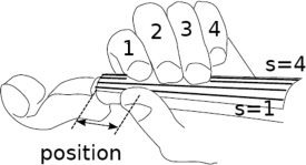
Figure 1. Violin fingering.
Violin Fingering: A Primer
We shall briefly review the fundamentals of violin
fingering and its terminology, as these play impor-
tant roles in understanding our method. The left
hand defines the pitch and the string on which a
note is played. Although there are two defining
factors in fingering (i.e., finger and string), violinists
often talk about fingering also in terms of the left
hand position, i.e., the general placement of the
left hand required to play a given note on a certain
string using a certain finger. As shown in Figure 1,
in this article we associate the string on which a
note is played with the variable s, where s = 1 is the
lowest-tuned string and s = 4 is the highest. These
strings are conventionally tuned seven semitones
apart, where s = 3 is typically tuned to A4 = 440 Hz.
The strings are typically notated in a music score
using a Roman numeral, where the lowest string
(s = 1) is associated with IV, and the highest (s =
4) with I. Placed fingers are labeled by numbers,
where 1 refers to the index finger, 2 the middle, 3
the ring, and 4 the little finger. An open string (i.e.,
no finger is pressed and the string vibrates at the
tuned pitch) is referred to by 0; only four pitches on a
violin can be played as an open string. In this article,
the position is defined by the number of semitones
that the first finger must traverse from the nut (the
ridge over which the string passes on the end of the
fingerboard near the tuning pegs) in order to play a
particular fingering.
Finger placement is determined by considering
technical ease and musical effect. Using a certain
finger (e.g., the index finger instead of the little
finger) facilitates execution of some musical effects
related to pitch, such as a smooth transition between
two notes (glissando), or a low-frequency modula-
tion of a note (vibrato). At the same time, some
sequences of finger placement are easier to execute
than others. For example, rapid movement of the
little finger is considerably more tiresome than that
of the index finger. The choice of the string on which
to play a given note is determined by considering the
consistency of sonority. For example, because each
string has a distinct sonority, violinists often play
on one string to prevent abrupt changes of the sound
quality. The difference in sonority when a given
pitch is played on one string versus another results
from (1) the differences in the physical attributes of
each string itself, such as the diameter, tension, and
material; (2) differences in the position along the
string at which the finger must be placed (because
each string is tuned differently); and (3) in cases
when the pitch is available as an open string, the
difference between the rigid termination provided
by the nut and the soft termination provided by the
finger.
The choice of string is the one factor in fingering
that is most likely to produce audible differences. By
contrast, the position is sometimes chosen for visual
effect and to demonstrate the violinist’s technical
skills. For example, the violinist may present a
“flashy” playing style through a wide change of
position.
The consistency of sonority offered by playing
on one string often forms a trade-off with the
consistency of position that facilitates playing. In
a fast piece, abrupt changes of sonority caused by a
certain fingering may be overlooked if it simplifies
playing. On the other hand, in a slow piece, a vio-
linist may choose a difficult fingering that produces
a certain sonority. A violinist may, for example,
value consistency of sonority in a slow, “singing”
(cantilena) passage by playing on one string.
Method
Our method is based on determining the fingerboard-
location sequence from a polyphonic audio mixture
that contains a musical phrase for solo violin, and
finding a sensible fingering that satisfies the esti-
mated fingerboard-location sequence. We assume
the violin plays a monophonic melody using normal
bowing technique (i.e., we do not consider extended
Maezawa et al.
59
l
D
o
w
n
o
a
d
e
d
f
r
o
m
h
t
t
p
:
/
/
d
i
r
e
c
t
.
m
i
t
.
e
d
u
/
c
o
m
j
/
l
a
r
t
i
c
e
–
p
d
f
/
/
/
/
3
6
3
5
7
1
8
5
7
1
0
0
/
c
o
m
_
a
_
0
0
1
2
9
p
d
.
j
f
b
y
g
u
e
s
t
t
o
n
0
7
S
e
p
e
m
b
e
r
2
0
2
3
Figure 2. System block
diagram.
playing technique such as plucking [pizzicato],
striking the string with the wooden side of the bow
[col legno],or playing very close to the bridge to
produce a shimmering sound [sul ponticello]).
Our task involves three aspects:
1. Designing a feature that performs well in a
polyphonic mixture.
2. Designing a scheme such that the perfor-
mance does not degrade from an acoustical
mismatch with the training data, whether
because of characteristics of the violins, the
rooms, or the recording process.
3. Designing a fingering model that reflects the
practices of violin performance.
We attack the first problem by fitting a sum-of-
sinusoids plus noise model to the observed spectrum
and using the estimated harmonic parameters as
the feature. The second problem is attacked by
normalizing the average features of the training
set and by doing the same for the recording whose
fingerboard-location sequence we would like to
identify. We solve the third problem by introducing a
new model of violin fingering, the violin pedagogical
model, which incorporates features that are inspired
by practices of violin playing. The system-level
block diagram is shown in Figure 2.
Fingerboard-Location Sequence Estimation
through Viterbi Alignment
In order to estimate a sensible fingering from the
audio, the fingerboard-location sequence must be
estimated from a polyphonic mixture of sound
that contains a violin melody. Because the string
on which a note is played (the bowed string) is
the primary factor that influences the timbre for
different fingerboard locations, we would like
to estimate the sequence of bowed strings. Our
estimation method is based on a bowed-string
classifier using features that are robust to polyphonic
accompaniment, and a classifier that takes into
account the playability of a particular fingerboard-
location sequence.
Feature Extraction by Harmonic-Model Fitting
We extract, from a polyphonic audio mixture that
contains a violin melody, the relative strengths of
the first N violin harmonics (partials), where N =
10, the first partial is the fundamental frequency,
and the others are overtones. The parameter is
dependent on the material property of the string,
the body resonance characteristics, and on how
the instrument is played (e.g., bow force, bow
velocity, and the contact point of the bow and
the string [Cremer and Allen 1984; Fletcher and
Rossing 1998]). The feature extraction involves
fitting a sum of harmonically spaced sinusoids
onto the observed short-time Fourier transform
representation of the input audio signal, Y( f , t),
where f is the frequency bin and t is the time index.
Because the input contains not only the harmonic
sound of the violin but also transients of the violin
and accompaniments, the harmonic sound of the
violin part must be segregated. This is achieved by
generating a time-frequency mask that passes the
harmonic component of the violin part, based on the
observed spectrogram, the music score given as a
60
Computer Music Journal
l
D
o
w
n
o
a
d
e
d
f
r
o
m
h
t
t
p
:
/
/
d
i
r
e
c
t
.
m
i
t
.
e
d
u
/
c
o
m
j
/
l
a
r
t
i
c
e
–
p
d
f
/
/
/
/
3
6
3
5
7
1
8
5
7
1
0
0
/
c
o
m
_
a
_
0
0
1
2
9
p
d
.
j
f
b
y
g
u
e
s
t
t
o
n
0
7
S
e
p
e
m
b
e
r
2
0
2
3
standard MIDI file (SMF), and the mapping between
positions in the SMF and the audio signal (audio-
score alignment). As a signal-processing front end,
we attenuate the DC component and emphasize the
high-frequency component by applying a two-tap,
high-pass filter with filter coefficients [1,–1]. Then
our method iterates the following steps for a fixed
number of iterations:
1. Update the time-frequency mask to segregate
the harmonic components of the violin part,
using the audio-score alignment and the
estimated fundamental frequency as the cue.
2. Estimate the fundamental frequency of
the violin melody, taking into account the
pitch notated in the score, the observed
spectrogram, and the audio-score alignment.
In the first step, we generate a time-frequency
mask, which approaches 1 for time-frequency bins
that contain the violin sound and 0 otherwise. We
incorporate the musical score information (from the
SMF) and the audio-score alignment to find which
bins are expected to contain the sound of the violin.
Audio-score alignment is determined by extracting
a time-sequence of chroma values from both the
audio and the SMF, and performing dynamic time-
warping between the chroma representation of the
audio and SMF to find the optimal path, using the
cosine distance as the metric between the audio
and the score, similar to the existing work of Hu,
Dannenberg, and Tzanetakis (2003).
Audio-score alignment gives the time-sequence of
the notated pitch of the violin part, ˆf0(t), for all time
points t. Given this, we simultaneously segregate
the violin part and estimate the fundamental
frequency of the violin part, f0(t). Our idea, similar
to Kameoka’s method (Kameoka, Nishimoto, and
Sagayama 2007), is to apply a mask that resembles
a comb filter to the spectrum centered about ˆf0(t)
to segregate the violin part. Using the segregated
signal, we re-estimate the fundamental frequency.
We then re-apply to the original spectrum the mask
with the updated fundamental frequency. We iterate
these two steps of fundamental frequency update
and violin-part segregation until the fundamental
frequency converges.
We first segregate the violin part by separating
the signal into two sub-signals—the violin part
and the residual (i.e., the rest of the signal). We
assume that the likelihood of observing the violin
part at frequency f is hv( f | f0(t)), and is of form
(cid:2)
f ), and we assume that the
πnN( f |nf0(t), σ 2
N
n=1
likelihood of observing the residual is hR( f ) and is of
form 1
F , where F is the number of frequency bins to
consider. πn is a multinomial variable that indicates
the relative strength of the nth partial. N(x|μ, σ 2)
is the likelihood of x for a normal distribution
with mean μ and variance σ 2. We assume that the
likelihood of observing the violin part is α, and the
likelihood of observing the residual is 1−α. For each
frequency bin, we associate a latent variable ZV,
which indicates whether the violin or the residual
contributed to the observed power. ZV( f , t) = 1
indicates that at time t, the power contained in
frequency f originated from the violin part, and
ZO( f , t, n) = 1 indicates that, of frames generated
from the violin, it originated from the nth partial of
the violin part. The joint likelihood of the observed
signal and the latent variable is given as follows:
p(X( f , t), Z( f , t)| f0(t), α, π )
=
(cid:3)
f ,t
N(cid:3)
n=1
((1 − α)hR( f ))X( f ,t)(1−ZV( f ,t))
(cid:4)
(cid:4)
απnN
f |nf0(t), σ 2
f
(cid:5)(cid:5)
X( f ,t)ZV( f ,t)ZO( f ,t,n)
We optimize this model using the expectation-
maximization (EM) algorithm, in a manner similar
to the work of Kameoka, Nishimoto, and Sagayama
(2007). In the E-step, we use the parameter from the
previous step to find the distribution of Z given X
and the parameters. We assign the following:
QO( f , t, n) = p(Zn|X, f0, α, π )
=
Qv( f , t) =
(cid:2)
πnN( f |nf0(t), σ 2
f )
π ˜nN( f | ˜n f0(t), σ 2
f )
˜n
(cid:2)
n
α(t)
(1− α(t))hR( f ) + α(t)
πnN( f |nf0(t), σ 2
f )
πnN( f |nf0(t), σ 2
f )
(cid:2)
n
Maezawa et al.
61
l
D
o
w
n
o
a
d
e
d
f
r
o
m
h
t
t
p
:
/
/
d
i
r
e
c
t
.
m
i
t
.
e
d
u
/
c
o
m
j
/
l
a
r
t
i
c
e
–
p
d
f
/
/
/
/
3
6
3
5
7
1
8
5
7
1
0
0
/
c
o
m
_
a
_
0
0
1
2
9
p
d
.
j
f
b
y
g
u
e
s
t
t
o
n
0
7
S
e
p
e
m
b
e
r
2
0
2
3
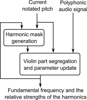
Figure 3. Block diagram of
feature extraction step.
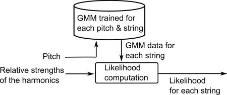
Figure 4. Block diagram of
the GMM.
l
D
o
w
n
o
a
d
e
d
f
r
o
m
h
t
t
p
:
/
/
d
i
r
e
c
t
.
m
i
t
.
e
d
u
/
c
o
m
j
/
l
a
r
t
i
c
e
–
p
d
f
/
/
/
/
3
6
3
5
7
1
8
5
7
1
0
0
/
c
o
m
_
a
_
0
0
1
2
9
p
d
.
j
f
b
y
g
u
e
s
t
t
o
n
0
7
S
e
p
e
m
b
e
r
2
0
2
3
n=1 X( f )QV( f , t)QO( f , t, n)n f df
˜n=1 X( f )QV( f , t)QO( f , t, ˜n) ˜n2 df
p(s = i|π (t), p(t), (cid:5)GMM( f0(t)))
In the M-step, we update the fundamental
frequency. We incorporate the knowledge that
the fundamental frequency does not deviate too
much from the notated pitch, by incorporating a
prior distribution of the fundamental frequency
as p( f0(t)| ˆf0(t)) = N( f0(t)| ˆf0(t), σ 2
yields the following updates:
f ). Then, the M-step
(cid:6)
(cid:2)
σ 2
f
ˆf0
+ σ 2
ˆf
(cid:6)
+ σ 2
σ 2
f
ˆf
F
(cid:2)
F
(cid:6)
F X( f )QV( f , t)QO( f , t, n) df
(cid:6)
F X( f )QV( f , t)QO( f , t, ˜n) df
(cid:6)
(cid:2)
˜n
F X( f )QV( f , t) df
F X( f ) df
(cid:6)
f0 : =
πn : =
α(t) =
A block diagram of this method is shown in
Figure 3.
Finally, we take the logarithm of π (t) to enable
feature adaptation, as will be discussed. Further-
more, we decorrelate the log-relative strength
by taking the discrete cosine transform. That is,
π (t) : = DCT(log π (t)).
Bowed String Identification
Once we extract the parameters (cid:5)(t) = { f0(t), π (t)},
we find the likelihood of the observed data for each
of the four bowed strings, i.e., the probability at each
point in time that the violinist is bowing a given
string.
The likelihood of bowed string si is modeled
using a Gaussian mixture model (GMM). The
GMM models the density of π for each pitch
pi( f0), where pi( f ) converts frequency f into the
closest MIDI note number. Let φ(i)
j ( p), and
(cid:2)
(i)
j ( p) indicate respectively the weight, the mean,
j ( p), μ(i)
and the covariance of the jth component of the
GMM for the ith bowed string at pitch p. Then,
the likelihood of observing bowed string i given
the feature { f0(t), π (t)} and the GMM parameters
θGMM = {φ(i)
follows:
j ( p)|∀i, j, p} is given as
j ( p), μ(i)
j ( p), σ (i)
(cid:7)
∝
j (pi(t))N(π (t)|μ(i)
φ(i)
j (pi(t)), (cid:8)(i)
j (pi(t))
j
θGMM is trained using violin audio examples with
various playing styles, each of which has a known
sequence of pitch and fingerboard position. Using
examples with a variety of playing styles has the
effect of averaging out statistical discrepancies of
the feature arising from playing the example in a
particular playing style. Hence, different parameters
in GMM correspond to timbral difference arising
from the variety of fingerboard position and pitch
combinations, and not playing style, e.g., bow
pressure or bow velocity. Figure 4 shows the block
diagram of the GMM.
The log-likelihood of the bowed string for the kth
note, then, is a sum of bowed-string likelihoods for
all audio frames that play the kth note. Let Tk(t) be
a binary variable that is 1 if frame t plays the kth
62
Computer Music Journal
Figure 5. Block diagram of
the HMM.
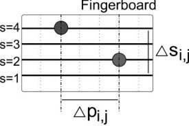
Figure 6. Simplified
horizontal–vertical model
used in the Viterbi
algorithm.
probability of the HMM. Then, we find the most
likely bowed string as follows:
ˆS = arg max
S={s0,···,sN}
p(S|(cid:5); (cid:5)GMM, v)
= arg max
(cid:7)
S={s0,···,sN}
log ρ0(s0) + log p(s0; v)
+
log p(si|si−1; v) + log ρi(si)
note notated on the score. Then, the bowed string
likelihood at note k, ρk(s), is given as follows:
ρk(s) =
(cid:7)
t
Tk(t) log p(s|π (t), p(t), θGMM)
Sequence Estimation using the Viterbi Algorithm
We determine the fingerboard-location sequence by
finding the most likely bowed-string sequence, tak-
ing into account the observed acoustic signal and the
difficulty of traversing from one fingerboard location
to another. To incorporate both the likelihood of a
given bowed string sequence and the likelihood of
observing the features given a particular fingerboard
position in which a note is played, we model the
bowed-string sequence as an HMM. Figure 5 shows
a graphical depiction of our model.
We treat the string the note is played on as the
hidden state that needs to be estimated, given the
observed features π (t), the fundamental frequency
f0(t), and the inherent difficulty from traversing
from one fingerboard position to another. Let v
be a parameter that governs the state transition
i=1
ρi(si) is the likelihood of the GMM obtained in the
previous section, for the ith note. The maximum-
likelihood sequence is determined inductively,
using the Viterbi algorithm. Let Sopt(m, s|X, (cid:5)) be
the optimal bowed-string sequence for the first m
notes that ends in bowed string s. Then, we define
Sopt(m+ 1, s|X, (cid:5)) as follows:
Sopt(m+ 1, s|π , (cid:5)) = log p(π (m+ 1)|s, (cid:5))
+ arg max
log p(Sopt(m, ˆs|π , (cid:5)))
ˆs
+ log p(s| ˆs, (cid:5))
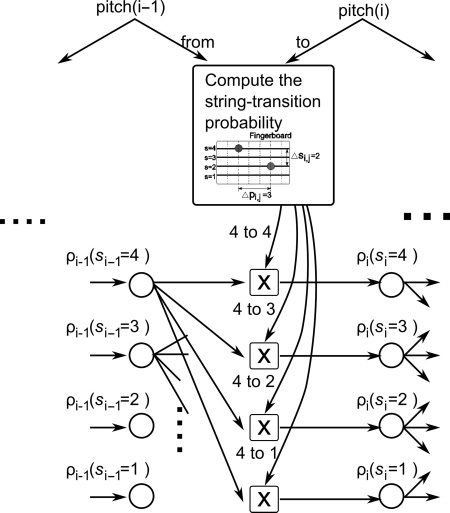
We design a suitable bowed-string transition
probability p(si|sj; v) based on a simplified violin
fingering model, as shown in Figure 6:
(cid:8)
(cid:8)(cid:9)
p(Si|Sj; v) ∝ exp
−v
(cid:11)(cid:11)
(cid:10)
2
(cid:10)pi, j
7
+ (cid:10)s2
i, j
Here, (cid:10)pi, j is the amount of change between
fingerboard positions and (cid:10)si, j is the amount of
change between string numbers. The constant
7 models the violinists’ tendencies to finger an
interval of up to 7semitones by either playing on the
same string or crossing a string, but to finger a larger
interval by crossing a string.
Maezawa et al.
63
l
D
o
w
n
o
a
d
e
d
f
r
o
m
h
t
t
p
:
/
/
d
i
r
e
c
t
.
m
i
t
.
e
d
u
/
c
o
m
j
/
l
a
r
t
i
c
e
–
p
d
f
/
/
/
/
3
6
3
5
7
1
8
5
7
1
0
0
/
c
o
m
_
a
_
0
0
1
2
9
p
d
.
j
f
b
y
g
u
e
s
t
t
o
n
0
7
S
e
p
e
m
b
e
r
2
0
2
3
Feature Adaptation
Fingering Estimation
Two violins typically sound different, mainly
because each violin has a unique body-resonance
characteristic. Therefore, it is essential for us to
adapt our model to violins with different body-
resonance characteristics.
Let Y1 and Y2 be the observed log-magnitude
spectrum of two violins. Let B1 and B2 be the
log-magnitude frequency response of the bodies
of the two violins, and S be the log-magnitude
spectrum of the bow-string interaction. Assum-
ing that the acoustic property of the bow–string
interaction does not change significantly across
different instruments, we obtain the following
relations:
Y1 = B1 + S
Y2 = B2 + S
S
+ (cid:4)Y2(cid:5)
X denotes expecta-
Taking the expectation, we obtain Y2 =
S, where (cid:4)Y(cid:5)
S is obtained readily by taking
S is
Y1 − (cid:4)Y1(cid:5)
tion of Y under probability distribution of X. In
our method, we let Y1 be the observed features,
and generate Y2, which is the feature when Y1 is
played on an instrument with body resonance char-
acteristic B2. (cid:4)Y1(cid:5)
the average of the observed signal, and (cid:4)Y2(cid:5)
obtained by summing the average feature of each
bowed string, weighted by how often a particu-
lar string is played at a given pitch for the given
music score. Because our features are linear trans-
formations of the logarithm of the relative powers
of harmonic peaks, the same rationale holds. Ini-
tially, we set the probability distribution of S as
follows:
p(S| pitch, β) ∼ exp
(cid:9)
− pitch − pitch0(S)
β
(cid:10)
if pitch > pitch0(S), 0 otherwise
Here, pitch is the played pitch, pitch0 is the
pitch of the open string played on string S, and
β is a positive parameter that assigns a greater
probability to lower fingerboard positions, which
are more commonly used and somewhat easier for
the violinist.
At the core of our fingering estimation is the violin-
fingering model, which models the difficulty of a
particular fingering. The fingering is determined by
designing a cost function between multiple states
of hand position, which reflects how difficult it
is for the hand to traverse from one position to
another.
Violin Fingering Model
In this study, we extend the existing horizontal–
vertical cost model presented in the previous section
to include fingering practices that are unique to the
violin, which we call the violin pedagogical model.
It is mainly inspired by practices of violin fingering
as suggested by Yampolsky (1967) and Flesch (Flesch
2000). The violin, in particular, is a small, unfretted
bowed stringed instrument, making it susceptible to
intonation errors. Hence, violin fingerings are often
set such that the weak finger (the little finger) is
used sporadically, and other fingers in such a way
that a natural hand position is maintained.
We define a fingering as a 4-tuple n = (n, s, f , p),
where n ∈ N is the pitch in MIDI note number,
s ∈ (1, 2, 3, 4) is the bowed string, f ∈ (0, 1, 2, 3, 4) is
the pressed finger (0 = open string, i.e., no finger
placed), and p ∈ N is the position. Let F be a set of all
possible fingerings. Also, let n(n) be a function that
retrieves the pitch of n ∈ F, s(n) the bowed string,
f(n) the finger, and p(n) the position.
We define an unnotated score, Su ∈ nM to be
an M−tuple of notes, where M is the number
of notes contained in the music score, and the
ith element, Su(i), is the ith note of the mu-
sic score. We define a bowed-string constraint,
cbow ∈ (1, 2, 3, 4)M associated with an unnotated
score Su as an M−tuple, where the ith element
indicates the bowed string for the ith note. We
finally define a notated score, Sn ∈ F M, where
the ith element contains the fingering for the ith
note.
We then formulate our problem as finding the
optimal notated score Sopt that satisfies both the
note sequence of the unnotated score obtained
using the SMF and the bowed-string constraint
64
Computer Music Journal
l
D
o
w
n
o
a
d
e
d
f
r
o
m
h
t
t
p
:
/
/
d
i
r
e
c
t
.
m
i
t
.
e
d
u
/
c
o
m
j
/
l
a
r
t
i
c
e
–
p
d
f
/
/
/
/
3
6
3
5
7
1
8
5
7
1
0
0
/
c
o
m
_
a
_
0
0
1
2
9
p
d
.
j
f
b
y
g
u
e
s
t
t
o
n
0
7
S
e
p
e
m
b
e
r
2
0
2
3
determined using the Viterbi algorithm. Namely,
we define cost functions for traversing a sequence of
two notes or three notes, and find the fingering with
the smallest net cost that satisfies the constraints.
Let Cb(si, si−1) : F 2 → R be a cost function defined
over a sequence of two notes. We define a symbol
Z that satisfies the following:
∀A ∈ F.Cb(Z, A) = Cb(A, Z) = 0
Then, the optimal fingering is a notated score Fopt
that satisfies the following:
Fopt = arg min
s1···sM∈F
M(cid:7)
i=1
Cb(si, si−1)
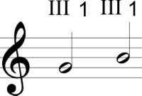
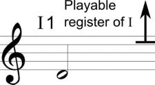
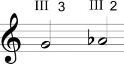
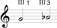
such that ∀ j < 1, ∀ j ∈ [1, M]n(si) = Su(i) sj = 0 and and s(Si) = cst(i) Let τp = 3, δi,j be Kronecker’s delta, and 1(c) be a function that is 1 if condition c is true and 0 otherwise. We define the following quantities for convenience: (cid:10)p(i, j) = p(si) − p(sj) (cid:10)s(i, j) = s(si) − s(sj) (cid:10)f(i, j) = f(si) − f(sj) (cid:10)pr(i, j) = |n(si) − p0(st(sj))| − |n(si) − p0(sj(sj))| R(i, j) = [Pmin(f(si), Pmax(f(sj))] Pmax = Pnat = ⎛ ⎜ ⎜ ⎜ ⎜ ⎜ ⎜ ⎝ ⎛ ⎜ ⎜ ⎜ ⎜ ⎜ ⎜ ⎝ ⎞ ⎟ ⎟ ⎟ ⎟ ⎟ ⎟ ⎠ ⎞ ⎟ ⎟ ⎟ ⎟ ⎟ ⎟ ⎠ 0 0 0 0 0 0 0 2 4 6 0 2 0 2 5 0 4 2 0 3 0 6 5 3 0 0 0 0 0 0 0 0 2 3 5 0 2 0 1 2 0 3 1 0 2 0 5 2 2 0 l D o w n o a d e d f r o m h t t p : / / d i r e c t . m i t . e d u / c o m j / l a r t i c e - p d f / / / / 3 6 3 5 7 1 8 5 7 1 0 0 / c o m _ a _ 0 0 1 2 9 p d . j f b y g u e s t t o n 0 7 S e p e m b e r 2 0 2 3 ⎛ ⎜ ⎜ ⎜ ⎜ ⎜ ⎜ ⎝ Pmin = 0 0 0 0 0 2.1 3.5 1 0 0 1.1 2.5 0 0 1 1.5 0 2.1 1.1 0 0 3.5 2.5 1.5 0 ⎞ ⎟ ⎟ ⎟ ⎟ ⎟ ⎟ ⎠ Then, we define a two-note generic fingering model (denoted HVM-2) as the following set of features XBN: b0 = |(cid:10)p(i, i − 1)| · 1(f(st) (cid:9)= 0 ∧ f(si−1) (cid:9)= 0) b1 = 1(fg(si) (cid:9)= 0 ∧ (cid:10)f(i, i − 1) = 0 ∧ (cid:10)p(i, i − 1) (cid:9)= 0) b2 = 1((cid:10)f(i, i − 1) · (cid:10)pr(i, i − 1) < 0 ∧ |(cid:10)p| < τp b3 = |(cid:10)pr(i, i − 1)| − Pnat(f(si), f(si−1)) ·1(|(cid:10)pr(i, i − 1)| ∈ R(i, i − 1)) xBN(1) = ∞ · 1(n(si) − p0(st(si)) − pos(si) /∈ R(1, i)) xBN(2, 3) = (b0, b2 0) xBN(4) = b1 xBN(5, 6) = (|(cid:10)s(i, i − 1)|, |(cid:10)s(i, i − 1)|2) ·1(fg(si) · fg(si−1) (cid:9)= 0) xBN(7) = 1(|(cid:10)pr(i, i − 1)| − Pnat(fg(si), fg(si−1)) (cid:9)= 0) xBN(8) = b2 · 1(fg(i) (cid:9)= 0 ∧ fg(i − 1) (cid:9)= 0) xBN(9) = b3 · 1(fg(i) = 0 ∨ fg(i − 1) = 0) xBN(1) determines whether a note is physically playable on a particular string, where ∞ × 0 = 0; i.e., this feature discards any fingering that is physically unplayable, as shown in Figure 7. xBN(2, 3) applies a penalty for a change of position. xBN(4) penalizes a change of position using the same finger (i.e., a glissando). xBN(5, 6) adds a penalty for a change of fingerboard location. xBN(7) penalizes playing in an unnatural hand position. xBN(8) penalizes playing a sequence in which the second note is placed higher on the fingerboard, but the finger traverses from high finger to low (e.g., little finger to the index finger), and vice versa. Finally, xBN(9) prevents change of Maezawa et al. 65 Figure 8. Graphical description of XBV(1). Figure 9. Graphical description of XBV(2). Figure 10. Graphical description of XBV(3). Figure 7. Graphical description of XBN(1). A Roman numeral indicates the string (IV = lowest, I = highest), and a number indicates the pressed finger (1 = index finger, 4 = little finger) Figure 7 Figure 8 l D o w n o a d e d f r o m h t t p : / / d i r e c t . m i t . e d u / c o m j / l a r t i c e - p d f / / / / 3 6 3 5 7 1 8 5 7 1 0 0 / c o m _ a _ 0 0 1 2 9 p d . j f b y g u e s t t o n 0 7 S e p e m b e r 2 0 2 3 Figure 9 Figure 10 lower-numbered finger, or vice versa, when the shift is small, as shown in Figure 10. xBV(4) penalizes an adjacent use of the little finger, which is weak and prone to intonation errors. xBV(5) adds a penalty for an extremely high position, which is harder to play in tune. xBV(6, 7) adds a preference for playing in the first, second, or third positions, which are typically the three easiest positions to play in. xBV(8) penalizes the half-position, the lowest possible position but an unconventional one; hence, it is unnatural from the perspective of violin pedagogy but perhaps the easiest position to play in tune from a physical perspective. Using these features, we define the two-note cost function as follows: Cb = diag(WBN WBV)[xBN xBV]T WBN and WBV define the relative weight of each feature. Given ample training data, statistical machine learning of these weights might be possible. In this article, we choose to manually adjust the weights, as the violin fingering corpus is too small to permit statistical machine learning. Experiments We perform three experiments. The first experiment assesses the performance of feature-adaptation and error-correction algorithms on bowed-string estimation, the second experiment assesses the performance of the bowed-string classifier in a position (wrist movement), when it is completely natural not to do so. We define a two-note fingering model inspired by the literature of violin pedagogy (denoted VPM-2) as the following set of features xBV: cond0 = fg(si) · fg(si−1) (cid:9)= 0 ∧ |(cid:10)p(i, i − 1)| < τp xBV(1) = 1(cond0 ∧ (cid:10)pr(i, i − 1) (cid:9)= 0 ∧ (cid:10)f(i, i − 1) = 0) xBV(2) = 1(cond0 ∧ |(cid:10)pr(i, i − 1)| = 1 ∧ |(cid:10)f(i, i − 1)| > 1)
xBV(3) = 1(fg(si) · fg(si−1) (cid:9)= 0 ∧ (cid:10)p(i, i − 1)
(cid:9)= 0 ∧ (cid:10)pr(i, i − 1) · (cid:10)f(i, i − 1) = −1)
xBV(4) = 1(fg(si) = fg(si−1)
= 4 ∧ |note(i) − note(i − 1)| > 1)
xBV(5) = pos(si)
xBV(6, 7, 8) = (δ2,pos(si), δ5,pos(si), δ1,fg(si))
xBV(1) penalizes using the same finger to move
to a different position, as shown in Figure 8. xBV(2)
penalizes a chromatic change of the relative position
using a nonadjacent finger, as shown in Figure 9;
such movement involves wrist motion, which is
considerably harder to tune than placing a finger
with a slight stretch. xBV(3) lessens the penalty
for shifting up from a higher-numbered finger to a
66
Computer Music Journal
Figure 11. Recognition
accuracy (%) for different
values of v (all values are
for data with data
adaptation). SS = same
violin and same strings as
training data; SD = same
violin with different
strings; DD = different
violin and different strings.
polyphonic mixture, and the third experiment
evaluates the playability of our new fingering model
through subjective experiments. In the first two
experiments, we prepared recordings of three pieces
of classical music, using two significantly different
fingerings (207 notes for three pieces, yielding a total
of 414 notes). For each fingering, we recorded the
music with the following three conditions:
1. Using the same violin and strings as were
used to record the training data (denoted as
setup SS).
2. Using the same violin but with a different
brand of strings (setup SD).
3. Using a different violin with a different brand
of strings (setup DD).
This results in about 18 minutes of audio for
validation. The training data, which lasts about 24
minutes, consists of two-octave chromatic scales
played on each string of an electric violin, using
various dynamics.
Setup SS and SD were played on the same electric
violin, and DD on an acoustic violin. We chose to
record the training data using an electric violin and
to use an acoustic violin for DD for two reasons.
First, it is easy to record noise-free training data
using an electric violin. Second, because electric
and acoustic violins sound extremely different, the
evaluation of the feature adaptation mechanism
can be regarded as the worst-case performance.
Therefore, in a real-life application, we expect the
system to perform somewhere between setup SD
and DD, as long as the training data use an acoustic
= 0.1 and σ2
violin. In the EM algorithm, we set σ 2
f
ˆf
to start at 50 and narrow down inverse-linearly with
each iteration of the algorithm. The value β used in
model adaption is chosen to be 0.1.
Experiment 1: Evaluation of Bowed-String
Identifier
We evaluated the accuracy of the bowed-string
estimator with and without feature adaptation, each
time evaluating the accuracy (1) of a baseline, i.e.,
without considering any sequential information; (2)
considering sequential information using a previous
study (Maezawa et al. 2009, 2010); and (3) considering
sequential information using the Viterbi algorithm
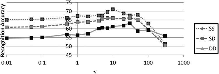
as proposed in this article. The value of v used for the
Viterbi algorithm in the bowed sequence estimation
was set to 30, chosen by evaluating the accuracy
for various values of v, as shown in Figure 11.
Figure 12 shows the result. We find that our method
consistently outperforms our previous study. In
all cases, adaptation decreases the performance
when the training data and the validation data are
from the same instrument and the same brand of
strings. This is because adaptation itself depends
on the estimated sequence of fingerboard positions,
which contains errors; the discrepancy between
the actual sequence of fingerboard positions and
the estimated ones is small enough to be effective
in absorbing the differences in body resonance
characteristics between two different violins or
strings, but significant when the same string and
violin is used.
Maezawa et al.
67
l
D
o
w
n
o
a
d
e
d
f
r
o
m
h
t
t
p
:
/
/
d
i
r
e
c
t
.
m
i
t
.
e
d
u
/
c
o
m
j
/
l
a
r
t
i
c
e
–
p
d
f
/
/
/
/
3
6
3
5
7
1
8
5
7
1
0
0
/
c
o
m
_
a
_
0
0
1
2
9
p
d
.
j
f
b
y
g
u
e
s
t
t
o
n
0
7
S
e
p
e
m
b
e
r
2
0
2
3
Figure 12. Comparison of
recognition accuracy (%)
for different sequence
estimation methods.
SS = same violin and
same strings as training
data; SD = same violin
with different strings;
DD = different violin and
different strings.
Figure 13. Recognition
accuracy with different
levels of accompaniment.
SS = same violin and same
strings as training data;
SD = same violin with
different strings;
DD = different violin
and different strings.
Figure 12
violin is greater than the “noise” level (i.e., the
accompaniment).
Experiment 3: Subjective Evaluation
of the Fingering Estimation
First, ten excerpts from three classical pieces were
prepared (approximately 200 notes total). For each
excerpt, we generated two fingerings: one using
HVM-2, and the other using HVM-2+VPM-2.
We assume that bowed-string estimation is per-
fectly accurate, by not incorporating constraints
based on the estimated bowed string. The feature
weight W was manually tuned, by first adjusting
the parameters for example (1) until it generated
satisfactory fingerings for the repertoires consid-
ered. Then, parameters pertaining to example (2)
were adjusted. They were set to WBN = [1, 0.5,
1, 1, 5, 1, 0.5, 20, 10] and WBV = [1, 10, –0.5, 10,
1.1, –0.3, –0.2, 0.2]. Excerpts that generated dif-
ferent fingerings for each of the setups were then
extracted.
Next, seven violinists of various skills (amateur
and professional, i.e., ten or more years of experience)
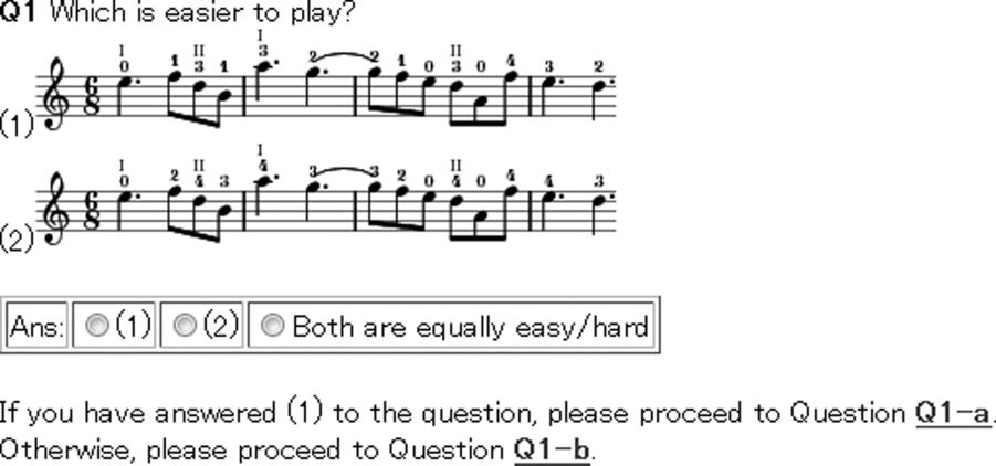
evaluated the generated fingerings using a form as
shown in Figure 14. Each violinist was presented
with fingerings generated using VPM-2 and VPM-2
+HVM-2, and was asked to choose the better of
the two, if any. Seven violinists were each given
ten questions (70 total), but only 66 answers were
Figure 13
Experiment 2: Effect of Accompaniment
on Feature Extraction
Piano accompaniments were generated for two of
the three pieces, using a synthesizer with uniform
note velocity, and the amplitude was adjusted such
that the peak values of the solo violin and the ac-
companiment were identical. Next, the recognition
accuracy was evaluated for each violin/string type,
by changing the level of the accompaniment. We
scaled the amplitude of the violin part such that the
root-mean-square power of the violin part relative
to that of the accompaniment is set to a given value
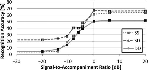
of signal-to-accompaniment ratio. Figure 13 shows
the result. We find that the bowed-string estimator
performs similarly for different ratios, as long as
the ratio is positive, that is, the signal level of the
68
Computer Music Journal
l
D
o
w
n
o
a
d
e
d
f
r
o
m
h
t
t
p
:
/
/
d
i
r
e
c
t
.
m
i
t
.
e
d
u
/
c
o
m
j
/
l
a
r
t
i
c
e
–
p
d
f
/
/
/
/
3
6
3
5
7
1
8
5
7
1
0
0
/
c
o
m
_
a
_
0
0
1
2
9
p
d
.
j
f
b
y
g
u
e
s
t
t
o
n
0
7
S
e
p
e
m
b
e
r
2
0
2
3
Figure 14. A screen capture
of the questionnaire.
Table 1. The Number of Answers Indicating a
Preference for the Baseline Model (HVM-2) or for
the Violin Pedagogical Model (HVM-2 + VPM-2)
Setup
HVM-2
HVM-2 + VPM-2
No preference
Total Count
5
54
7
provided. Table 1 shows the result of the survey. The
sign test shows that HVM-2 and VPM-2+HVM-2
are not equally favored ( p = 0.01), which suggests
that our proposed model (HVM-2+VPM-2) is favored
over the baseline (HVM-2 only).
Discussion
From the results in Experiment 1 we observe that in
setup DD—the most realistic situation—adaptation
improves the recognition accuracy, whereas in
SS and SD, the accuracy decreases. We believe
this occurs because of the mismatch between the
distribution of the actual bowed-string sequence
and that assumed in our model. Moreover, we find
that our study offers major improvements compared
with our previous study. In all cases, our method
improves the recognition accuracy over the baseline,
which suggests that considering the playability of
a particular sequence of notes over a particular
sequence of bowed strings is effective.
Experiment 2 suggests that our features are
robust in polyphonic audio mixtures, as long as the
signal level of the violin solo part is as loud as the
accompaniment. This condition seems to hold in
pieces where the violin has an important melody
(and hence, the choice of fingerboard location
becomes an even greater musical issue). Therefore,
we believe our method performs without significant
degradation of accuracy in practical applications
involving works for violin and piano.
Finally, we found that the fingering generated is
more natural when the proposed fingering model
is used than when existing ones are. We believe
incorporating the preference for the first and third
positions (index finger placed 2 semitones and 5
semitones above the nut of the violin, respectively)
is the chief reason—they are the most frequently
used positions on the violin, and fingerings generated
on these positions are more natural for violinists
to play. We find that incorporating these kinds of
heuristics could drastically improve playability.
Maezawa et al.
69
l
D
o
w
n
o
a
d
e
d
f
r
o
m
h
t
t
p
:
/
/
d
i
r
e
c
t
.
m
i
t
.
e
d
u
/
c
o
m
j
/
l
a
r
t
i
c
e
–
p
d
f
/
/
/
/
3
6
3
5
7
1
8
5
7
1
0
0
/
c
o
m
_
a
_
0
0
1
2
9
p
d
.
j
f
b
y
g
u
e
s
t
t
o
n
0
7
S
e
p
e
m
b
e
r
2
0
2
3
Figure 15. Estimated
fingering from first 50 bars
of Romanze in C played by
Joachim (1903).
l
D
o
w
n
o
a
d
e
d
f
r
o
m
h
t
t
p
:
/
/
d
i
r
e
c
t
.
m
i
t
.
e
d
u
/
c
o
m
j
/
l
a
r
t
i
c
e
–
p
d
f
/
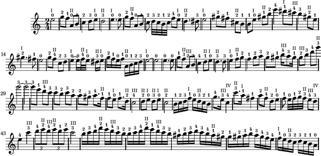
Next, we shall discuss an application of our
system for recovering the fingering of a recording
from more than a century ago.
had to have been played by stopping a string with
a finger. These kinds of errors might have occurred
for three reasons:
/
/
/
3
6
3
5
7
1
8
5
7
1
0
0
/
c
o
m
_
a
_
0
0
1
2
9
p
d
.
j
Application: Demystifying Historical Recordings
Our method may be used to analyze a recording
from the past to recover the fingering of a legendary
violinist. In this example, we attempt to recover the
fingering of Romanze in C composed by Joachim,
a legendary violinist of the late 19th century, using
a gramophone recording of Joachim in 1903. The
recording was pitch-shifted such that the notated A4
was set to 440 Hz. VPM-2+HVM-2 fingering model
was used to estimate the fingering, an excerpt of
which is shown in Figure 15.
We speculate, however, that the actual fingering
may have been very different from that estimated
by our method. For example, there are notes that are
playable using open strings (i.e., no finger pressed)
whose estimated fingerings on the notated score
show open strings; yet, on the recording, we clearly
hear the note played with a vibrato, meaning that it
f
b
y
g
u
e
s
t
t
o
n
0
7
S
e
p
e
m
b
e
r
2
0
2
3
A) In Joachim’s time, the material used for the
violin string was significantly different. In
particular, the E-string (the highest-pitched
string) used gut as its core, which has a much
mellower timbre than the kind of string used
today. Such discrepancies in the material
property of the string itself would cause the
performance of the bowed-string estimator
to deteriorate.
B) A high-quality recording of Joachim is not
available. The remastered recording we used
had a frequency range that extended up to
only approximately 5 kHz; the rest was cut
off, perhaps by applying an equalizer. Hence,
there were only few partials that conveyed
meaningful information.
C) Joachim’s use of pitch-based playing tech-
niques, such as vibrato and glissando, gives
many clues to violinists who want to infer
Joachim’s playing. For example, if a transition
70
Computer Music Journal
from one note to another is completely
smooth, it strongly suggests that the two
notes were played on the same string. Vibrato
can be a giveaway for distinguishing whether
a note is played using an open string or not.
Our method, however, does not incorporate
the pitch trajectory for fingerboard-location
estimation, and hence, misses such clues.
This output suggests a future direction for
research: incorporating pitch-based cues for finger-
board inference, and perhaps robustness to differ-
ent materials used for a given string. The latter,
however, can be ameliorated with our method to a
certain extent; we can record the training data using
the string that is thought to be used in the recording
whose fingering we would like to infer.
On Inharmonicity
Stringed instruments such as the violin do not
produce overtones that are exact integer multiples
of the fundamental frequency. Such deviation from
integer harmonics is caused by the inharmonicity
of the violin string, which in turn is created
by torsion of the string. Because inharmonicity
is dependent on the material of the string, our
model initially incorporated inharmonicity, using
a beta distribution with a small shape parameter
as its prior distribution. We found, however, that
such a model produced lower accuracy than that
without inharmonicity. Because of the nature of
the EM algorithm, we found that the model tends
to “explain” partials of the accompaniment as
arising from the violin sound with extremely high
inharmonicity.
Conclusion
mixture. We also incorporated a sequential model
based on violin playing. We found that such sequen-
tial modeling drastically improved the accuracy. The
fingering estimation incorporated features that are
specific to violin playing practices (the pedagogical
model), in addition to some of the more fundamen-
tal features applicable to other instruments as well.
Incorporating such heuristics generated a drastically
easier fingering.
Future research directions may involve improved
recognition accuracy, refining the fingering model,
and more applications. For example, recognition ac-
curacy may be improved by exploiting the smooth-
ness of pitch trajectory (glissando, vibrato, etc.), as
we observed that violinists listen to the smoothness
of pitch transition to infer the fingerboard location
and the fingering. The fingering model may further
be improved by incorporating more features that are
inspired from violin pedagogy or through machine
learning of feature weights by preparing a large
violin fingering corpus. Another possibility is to
perform joint estimation of fingerboard location
and fingering—the problems of fingerboard location
estimation and fingering estimation are dependent
on each other, suggesting that joint estimation
may improve the performance of both. From a
musicological perspective, artist classification, skill
assessment, and analysis of historical recordings
may be interesting applications of our approach to
fingering estimation.
Acknowledgments
This work is supported by Grant-in-aid for Scientific
Research (S) and CREST-MUSE of JST.
We would like to thank violinists P. Klinger,
Dr. P. Sunwoo, and Dr. J. Choi for stimulating and
inspiring discussions on violin fingering.
This article presented a method for recovering the
violin fingering from an input audio signal and a
music score by analyzing the bowed-string sequence,
and using it as a constraint to determine the optimal
fingering. Bowed-string sequence classification was
based on features that are robust in a polyphonic
References
Barbancho, I. 2009. “Transcription and Expressiveness
Detection System for Violin Music.” In Proceedings of
the International Conference on Acoustics, Speech and
Signal Processing, pp. 189–192.
Maezawa et al.
71
l
D
o
w
n
o
a
d
e
d
f
r
o
m
h
t
t
p
:
/
/
d
i
r
e
c
t
.
m
i
t
.
e
d
u
/
c
o
m
j
/
l
a
r
t
i
c
e
–
p
d
f
/
/
/
/
3
6
3
5
7
1
8
5
7
1
0
0
/
c
o
m
_
a
_
0
0
1
2
9
p
d
.
j
f
b
y
g
u
e
s
t
t
o
n
0
7
S
e
p
e
m
b
e
r
2
0
2
3
Burns, A. M., and M. M. Wanderley. 2006. “Visual Methods
for Retrieval of Guitarist Fingering.” In Proceedings
of the International Conference on New Interface for
Musical Expression, pp. 196–199.
Cremer, L., and J. S. Allen. 1984. The Physics of the Violin.
Maezawa, A., et al. 2009. “Bowed String Sequence
Estimation of a Violin Based on Adaptive Audio
Signal Classification and Context-Dependent Error
Correction.” In Proceedings of the International
Symposium on Multimedia, pp. 9–16.
Cambridge, Massachusetts: MIT Press.
Flesch, C. 2000. The Art of Violin Playing. 2nd ed., vol. I.
New York: Carl Fischer.
Fletcher, N. H., and T. D. Rossing. 1998. The Physics of
Musical Instruments. 2nd ed. New York: Springer.
Hu, N., R. B. Dannenberg, and G. Tzanetakis. 2003.
“Polyphonic Audio Matching and Alignment for Music
Retrieval.” In Proceedings of the Institute of Electrical
and Electronics Engineers Workshop on Applications
of Signal Processing to Audio and Acoustics, pp. 185–
188.
Kameoka, H., T. Nishimoto, and S. Sagayama. 2007. “A
Multipitch Analyzer Based on Harmonic Temporal
Structured Clustering.” Institute of Electrical and
Electronics Engineers Transactions on Audio, Speech
and Language Processing 15(3):982–994.
Kasimi, A. A., E. Nichols, and C. Raphael. 2007. “A Simple
Algorithm for Automatic Generation of Polyphonic
Piano Fingerings.” In Proceedings of the International
Society for Music Information Retrieval Conference,
pp. 355–356.
Krishnaswamy, A., and J. Smith. 2003. “Inferring Control
Inputs to an Acoustic Violin from Audio Spectra.” In
Proceedings of the Institute of Electrical and Electronics
Engineers International Conference on Multimedia and
Expo, pp. 733–736.
Lu, H., et al. 2008. “iDVT: An Interactive Digital Violin
Tutoring System Based on Audio-Visual Fusion.”
In Austria Association for Computing Machinery
International Conference on Multimedia, pp. 300–
301.
Maezawa, A., et al. 2010. “Violin Fingering Estimation
Based on Violin Pedagogical Fingering Model Con-
strained by Bowed Sequence Estimation from Audio In-
put.” Trends in Applied Intelligent Systems, 3:249–259.
Radicioni, D. P., L. Anselma, and V. Lombardo. 2004.
“A Segmentation-Based Prototype to Compute
String Instruments Fingering.” In Proceedings of the
Conference on Interdisciplinary Musicology. Available
online at www.uni-graz.at/richard.parncutt/cim04.
Accessed May 2012.
Radisavljevic, A., and P. F. Driessen. 2004. “Path
Difference Learning for Guitar Fingering Problems.”
In Proceedings of the International Computer Music
Conference, pp. 730–733.
Sayegh, S. I. 1989. “Fingering for String Instruments with
the Optimal Path Paradigm.” Computer Music Journal
13(3):76–83.
Traube, C., and J. Smith. 2000. “Estimating the Plucking
Point on a Guitar String.” In Proceedings of the Interna-
tional Conference on Digital Audio Effects, pp. 153–158.
Yampolsky, I.M. 1967. Principles of Violin Fingering. New
York: Oxford University Press.
Yonebayashi, Y., H. Kameoka, and S. Sagayama. 2007.
“Automatic Decision of Piano Fingering Based
on a Hidden Markov Model.” In Proceedings of
the International Joint Conference on Artificial
Intelligence, pp. 2915–2921.
Zhang, B., J. Zhu, and W. Leow. 2007. “Visual Analysis
of Fingering for Pedagogical Violin Transcription.” In
Proceedings of the ACM Conference on Multimedia,
pp. 521–524.
72
Computer Music Journal
l
D
o
w
n
o
a
d
e
d
f
r
o
m
h
t
t
p
:
/
/
d
i
r
e
c
t
.
m
i
t
.
e
d
u
/
c
o
m
j
/
l
a
r
t
i
c
e
–
p
d
f
/
/
/
/
3
6
3
5
7
1
8
5
7
1
0
0
/
c
o
m
_
a
_
0
0
1
2
9
p
d
.
j
f
b
y
g
u
e
s
t
t
o
n
0
7
S
e
p
e
m
b
e
r
2
0
2
3