INVESTIGACIÓN
A covariate-constraint method to map brain
feature space into lower dimensional manifolds
Félix Renard1, Christian Heinrich2, Marine Bouthillon2, Maleka Schenck3,4,
Francis Schneider3,4,5, Stéphane Kremer2,6, and Sophie Achard 1
1Université Grenoble Alpes, CNRS, Inria, Grenoble, Francia
2iCube, Université de Strasbourg, CNRS, Illkirch, Francia
3Service de Médecine Intensive Réanimation, CHU de Strasbourg, Francia
4Faculté de Médecine FMTS, Strasbourg, Francia
5U1121, Université de Strasbourg, Francia
6Imagerie 2, CHU de Strasbourg, Université de Strasbourg, Francia
Palabras clave: Graphs, Machine learning, Connectomes, Hub disruption index
ABSTRACTO
Human brain connectome studies aim to both explore healthy brains, and extract and
analyze relevant features associated with pathologies of interest. Usually this consists of
modeling the brain connectome as a graph and using graph metrics as features. A fine brain
description requires graph metrics computation at the node level. Given the relatively
reduced number of patients in standard cohorts, such data analysis problems fall in the
high-dimension, low-sample-size framework. In this context, our goal is to provide a
machine learning technique that exhibits flexibility, gives the investigator an understanding of
the features and covariates, allows visualization and exploration, and yields insight into the
data and the biological phenomena at stake. The retained approach is dimension reduction
in a manifold learning methodology; the originality is that the investigator chooses one (o
varios) reduced variables. The proposed method is illustrated in two studies. The first one
addresses comatose patients; the second one compares young and elderly populations. El
method sheds light on the differences between brain connectivity graphs using graph metrics
and potential clinical interpretations of these differences.
RESUMEN DEL AUTOR
Human brain connectome studies aim at both exploring healthy brains, and analyzing
relevant features associated to pathologies of interest. This consists in modeling the brain
connectome as a graph and in using graph metrics as features. Such data analysis problems
fall in the high-dimension low sample size framework. Our goal is to provide a machine
learning technique that exhibits flexibility, gives the investigator grip on the features and
covariables, allows visualization, and yields insight into the biological phenomena at stake.
The retained approach is dimension reduction in a manifold learning methodology, el
originality lying in that several reduced variables be chosen by the investigator. The method
sheds light on the differences between brain connectivity graphs using graph metrics and
potential clinical interpretations of theses differences.
un acceso abierto
diario
Citación: Renard, F., Enrique, C.,
Bouthillon, METRO., Schenck, METRO., Schneider,
F., Kremer, S., & Achard, S. (2021). A
covariate-constraint method to map
brain feature space into lower
dimensional manifolds. Red
Neurociencia, 5(1), 252–273.
https://doi.org/10.1162/netn_a_00176
DOI:
https://doi.org/10.1162/netn_a_00176
Información de apoyo:
https://doi.org/10.1162/netn_a_00176
https://github.com/renardfe/CCML
Recibió: 8 Puede 2020
Aceptado: 24 Noviembre 2020
Conflicto de intereses: Los autores tienen
declaró que no hay intereses en competencia
existir.
Autor correspondiente:
Félix Renard
felixrenard@gmail.com
Editor de manejo:
James Shine
Derechos de autor: © 2020
Instituto de Tecnología de Massachusetts
Publicado bajo Creative Commons
Atribución 4.0 Internacional
(CC POR 4.0) licencia
La prensa del MIT
yo
D
oh
w
norte
oh
a
d
mi
d
F
r
oh
metro
h
t
t
pag
:
/
/
d
i
r
mi
C
t
.
metro
i
t
.
t
/
/
mi
d
tu
norte
mi
norte
a
r
t
i
C
mi
–
pag
d
yo
F
/
/
/
/
/
5
1
2
5
2
1
9
1
1
5
7
4
norte
mi
norte
_
a
_
0
0
1
7
6
pag
d
t
.
F
b
y
gramo
tu
mi
s
t
t
oh
norte
0
7
S
mi
pag
mi
metro
b
mi
r
2
0
2
3
Mapping the brain feature space into lower dimensional manifolds
INTRODUCCIÓN
Brain modeling and understanding is a very active field of research involving different dis-
ciplines, such as neuroscience, image and signal processing, Estadísticas, física, y biología.
These last years, neuroimaging modalities have been developed to explore the brain for both
structural and functional features. It is now recognized that these images are providing very
promising noninvasive observations of the brain (bullmore & despreciar, 2009; Mwangi, tian, &
Órdenes, 2014; Richiardi, Achard, Montón, & Van De Ville, 2013). One consequence of the avail-
ability of such massive datasets is the need to develop more and more sophisticated models
to unravel the possible alteration of brains due to the impact of different pathologies. En esto
contexto, representing the brain as a global system is capital. This may be achieved using a
red (bullmore & despreciar, 2009). A brain network is a graph where nodes correspond to
specific regions, and edges describe interactions and links between those regions. Different
kinds of links and interactions may be of interest. Anatomical tracts are identified using dif-
fusion imaging (despreciar, Tononi, & kötter, 2005) and used in anatomical connectivity studies,
where the whole set of links is called an anatomical connectome. Functional interactions are
identified in functional imaging studies, whether in resting state or in task performing (Fallani,
Richiardi, Chavez, & Achard, 2014; Rosazza & Minati, 2011), and used in functional con-
nectivity studies. The whole set of functional links is called a functional connectome. En el
functional case, brain networks are particularly adequate in encapsulating both spatial and
temporal information in a single model. En efecto, brain networks are constructed using brain
parcellation, namely spatial features, and time series interactions, namely temporal features.
This model has attracted lots of attention these last 20 years by providing both very intuitive
and spatial maps of brain networks.
Brain networks can be quantified using graph metrics such as minimum path length, clus-
tering (vatios & Strogatz, 1998), global and local efficiency (latora & marchiori, 2001), modu-
larity (Hombre nuevo, 2006), and assortativity (Hombre nuevo, 2002), entre otros. As these metrics are
associated with specific network features, it is often possible to find the appropriate metrics
to use given specific neuroscience hypotheses of the study. For the study of brain disorders,
these metrics have been used in order to extract biomarkers for pathologies such as for ex-
ample Alzheimer’s disease (Supekar, menón, Frotar, Musen, & Greicius, 2008), schizophrenia
(Lynall et al., 2010), and multiple sclerosis (Filippi et al., 2014). Extracting quantitative param-
eters of brain networks is compulsory to conduct any statistical analysis. In this framework,
statistical and machine learning approaches on graph metrics on all nodes allow the quantifi-
cation of differences between groups (Richiardi et al., 2013).
For any dataset, any graph metric can be computed either at the global level with one value
for an entire network or at the nodal level with one value for each node and a vector of values
for the entire network. It has already been shown that global values may not discriminate two
groups of subjects (Achard et al., 2012), which shows their limits as biomarkers. Few attempts
have been made to directly use distances between networks such as the edit distance (Mokhtari
& Hossein-Zadeh,2013), or network similarities (Mheich et al., 2017). Sin embargo, nodal-level
approaches are challenging since hundreds of brain areas can be extracted whereas the num-
ber of subjects is generally small. This corresponds to the high-dimension, low-sample-size
(HDLSS) configuration and falls under the curse of dimensionality (Bellman, 1961). En el particular-
prolongada, standard classification and regression algorithms are not robust anymore in such a context
(Hastie, Ruidoso, & Friedman, 2001, Capítulo 2, Sección 5, y capítulo 18).
Dimension-reduction techniques tackle curse of dimensionality issues (Hastie et al., 2001).
In this framework, feature selection, where a subset of the original variables is considered, y
High-dimension, low-sample-size
(HDLSS) estructura:
HDLSS is a mathematical concept to
characterize a key challenge in data
análisis, mainly the difference
between the number of parameters
and the number of observations.
Neurociencia en red
253
yo
D
oh
w
norte
oh
a
d
mi
d
F
r
oh
metro
h
t
t
pag
:
/
/
d
i
r
mi
C
t
.
metro
i
t
.
t
/
/
mi
d
tu
norte
mi
norte
a
r
t
i
C
mi
–
pag
d
yo
F
/
/
/
/
/
5
1
2
5
2
1
9
1
1
5
7
4
norte
mi
norte
_
a
_
0
0
1
7
6
pag
d
t
.
F
b
y
gramo
tu
mi
s
t
t
oh
norte
0
7
S
mi
pag
mi
metro
b
mi
r
2
0
2
3
Mapping the brain feature space into lower dimensional manifolds
ISOMAP methodology:
ISOMAP is a dimension-reduction
methodology consisting of projecting
the initial observations to a reduced
espacio, where it is simpler to describe
and interpret the results.
κ or hub disruption index:
κ is a graph metric to quantify the
differences of locations of hubs and
non-hubs between a patient and a
group of controls.
feature extraction, where the original variables are transformed to a smaller set, may be envis-
aged (Webb, 2002). We resort here to the ISOMAP methodology, which is a well-known non-
linear feature extraction algorithm generalizing principal component analysis (PCA) dimensión
reducción (Huo, En, & Herrero, 2007; Tenenbaum, de Silva, & Langford, 2000). ISOMAP may be
seen as a manifold learning approach, where the degrees of freedom of the data are captured
by the latent variables, and where the structure of points in the latent space (the reduced space)
mimics the structure of data in the original space. Sin embargo, ISOMAP raises two issues:
interpreting the latent variables and determining the effect a change in the latent variables in-
curs in the data space; eso es, the corresponding changes in brain networks and the underlying
neuroscience hypotheses at stake in the case of the present study.
Dimension reduction is not new in the field of brain connectivity studies. Several methods
have been proposed to extract nodal features at the level of brain regions. Using the hub dis-
ruption index (the κ index) to analyze a set of brain networks may be considered a feature
extraction approach: This is a user-defined transformation of the original space to a 1D la-
tent space (Achard et al., 2012). Principal component analysis was previously applied on
graph metrics in Robinson, Hammers, Ericsson, Edwards, and Rueckert (2010) with vectors
representing brains at the nodal level. We proposed in Renard, Enrique, Achard, Hirsch,
and Kremer (2012) to use kernel PCA, a nonlinear version of PCA. Además, interpreting la-
tent variables may be addressed by correlating the reduced space with clinical data (Gerber,
Tasdizen, Thomas Fletcher, Joshi, & Whitaker, 2010). Covariates may also be mapped or re-
gressed on the reduced space as proposed in Aljabar, Wolz, and Rueckert (2012), thus shedding
light on latent variables. Dimension-reduction methods have also been applied to connectiv-
ity matrices (Ktena et al., 2018; Kumar, Toews, Chauvin, Colliot, & Desrosiers, 2018; Yamin
et al., 2019) or to the voxel time series (Saggar et al., 2018), mainly for classification purposes.
It is indeed difficult using the whole connectivity matrices or voxel time series to give an inter-
pretation at the nodal or voxel level (Gallos & Siettos, 2017; Haak, Marquand, & beckman,
2018; Laurienti et al., 2019). Network embedding framework can be viewed as a dimension-
reduction method and was also applied to brain connectivity graphs (Rosenthal et al., 2018).
yo
D
oh
w
norte
oh
a
d
mi
d
F
r
oh
metro
h
t
t
pag
:
/
/
d
i
r
mi
C
t
.
metro
i
t
.
/
t
/
mi
d
tu
norte
mi
norte
a
r
t
i
C
mi
–
pag
d
yo
F
/
/
/
/
/
5
1
2
5
2
1
9
1
1
5
7
4
norte
mi
norte
_
a
_
0
0
1
7
6
pag
d
t
.
The objective of this article is to integrate all features cited above in one method: working
at the nodal level, applying dimension-reduction techniques, and mapping covariates to ease
interpretación. Además, a new methodology is proposed to incorporate interesting network
features already identified in specific datasets directly in the manifold learning approach. Estafa-
trary to statistical tests at nodal levels where each feature is treated independently of others,
our approach based on machine learning is able to analyze joint variations between local
descriptors.
F
b
y
gramo
tu
mi
s
t
t
oh
norte
0
7
S
mi
pag
mi
metro
b
mi
r
2
0
2
3
This paper is focusing on two already published datasets. The first one consists of fMRI data-
sets on 20 healthy controls and 17 coma patients from Achard et al. (2012). The second one
is based on Achard and Bullmore (2007), dónde 15 young healthy subjects and 11 elderly
healthy subjects were scanned using resting-state fMRI. Our first experiment compares data-
driven approaches such as linear discriminant analysis (LDA) and random forests (RF) to an
ad hoc description such as the hub disruption index κ. This allows us to compare classical
machine learning approaches, in which the interpretability of the results is often difficult, con
approaches resorting to descriptors constructed using neuroscientific hypotheses. This first ex-
periment can be seen as preliminaries of the sequel of the paper, where a feature is extracted
for each individual in order to optimize classification of the two groups using either classi-
cal machine learning approaches or ad hoc descriptors. The second experiment consists of
constructing a data-driven manifold, ISOMAP, using the graph metrics as features. ISOMAP
Neurociencia en red
254
Mapping the brain feature space into lower dimensional manifolds
is providing a compact representation of brain connectomes in a reduced space, where it is
straightforward to map the available covariates. Además, we may interpret changes in con-
nectomes by regressing covariables like κ on the reduced space using latent variables.
This representation allows a visualization of each subject relative to the whole population,
which is crucial in clinical studies, for example in order to better understand brain changes for
each specific subject. Además, κ has been shown to be both a meaningful descriptor and
a good classifying feature for brain connectomes of coma patients. Por lo tanto, we propose a
new method based on a covariate-constrained manifold learning (CCML) using κ as an input
of ISOMAP. This allows us to propose a new generative model based on our new data rep-
resentimiento, to better predict the variation in each patient given the changes of covariables.
Based on the results of the first experiment, the choice of the covariate, κ in this work, can be
adjusted to the studied datasets.
MATERIALES Y MÉTODOS
Resting-State fMRI Data
The data were acquired in a previous study aimed at characterizing resting-
Comatose study.
state connectivity brain networks for patients with consciousness disorders. The description of
the data and results is reported in Achard et al. (2012). The patients were scanned a few days
after major acute brain injury, when sedative drug withdrawal allowed for spontaneous ventila-
ción. Por lo tanto, all patients were spontaneously ventilating and could be safely scanned at the
time of fMRI. The causes of coma are patient-dependent: 12 had cardiac and respiratory arrest
due to various causes; 2 had a gaseous cerebrovascular embolism; 2 had hypoglycemia; y 1
had extracranial artery dissection. Un total de 25 patients were scanned (age range, 21–82 years;
9 hombres). Data on eight patients were subsequently excluded because of unacceptable degrees
of head movement. The coma severity for each patient was clinically assessed using the 62
items of the WHIM scale: scores range from 0, meaning deep coma, a 62, meaning full recov-
ery. Six months after the onset of coma, 3 patients had totally recovered, 9 patients had died,
y 5 patients remained in a persistent vegetative state. The normal control group is composed
de 20 healthy volunteers matched to the group of patients for sex (11 hombres) y aproximadamente
for age (rango, 25–51 years). This study was approved by the local Research Ethics Commit-
tee of the Faculty of Health Sciences of Strasbourg on October 24, 2008, (CPP 08/53) and by
the relevant healthcare authorities. Written informed consent was obtained directly from the
healthy volunteers and from the next of kin for each of the patients. Resting-state data were
acquired for each subject using gradient echo planar imaging technique with a 1.5-T MR scan-
ner (Avanto; Siemens, Erlangen, Alemania) with the following parameters: relaxation time =
3 s, echo time = 50 EM, isotropic voxel size = 4 × 4 × 4 mm3, 405 imágenes, y 32 axial slices
covering the entire cortex. The preprocessing of the data is detailed in our previous study
(Achard et al., 2012).
The data used in this study have already been analyzed in two papers
Young and elderly study.
(Achard & bullmore, 2007, and Meunier, Achard, Morcom, & bullmore, 2009). The goal of
these papers was to identify the changes in brain connectomes for elderly subjects in terms of
topological organization of brain graphs. The data consist of 15 young subjects aged 18–33
años, edad media = 24 y 11 elderly subjects aged 62–76 years. Each subject was scanned
using resting-state fMRI as described in Achard and Bullmore (2007, Wolfson Brain Imaging
Centre, Cambridge, Reino Unido). For each dataset, un total de 512 volumes were avalaible with num-
ber of slices, 21 (interleaved); slice thickness, 4 mm; interslice gap, 1 mm; matrix size, 64 × 64;
Neurociencia en red
255
yo
D
oh
w
norte
oh
a
d
mi
d
F
r
oh
metro
h
t
t
pag
:
/
/
d
i
r
mi
C
t
.
metro
i
t
.
/
t
/
mi
d
tu
norte
mi
norte
a
r
t
i
C
mi
–
pag
d
yo
F
/
/
/
/
/
5
1
2
5
2
1
9
1
1
5
7
4
norte
mi
norte
_
a
_
0
0
1
7
6
pag
d
t
.
F
b
y
gramo
tu
mi
s
t
t
oh
norte
0
7
S
mi
pag
mi
metro
b
mi
r
2
0
2
3
Mapping the brain feature space into lower dimensional manifolds
flip angle, 90°; repetition time (TR), 1,100 EM; tiempo de eco, 27.5 EM; in-plane resolution,
3.125 mm.
Preprocessing and Wavelet Graph Estimation
Brain network graphs were determined following Achard et al. (2012) for the comatose study
and Achard and Bullmore (2007) for the young and elderly study. For each subject, data were
corrected for head motion and then coregistered with each subject’s T1-weighted structural
resonancia magnética. Each subject’s structural MRI was nonlinearly registered with the Colin27 template im-
edad. The obtained deformation field image was used to map the fMRI datasets to the automated
anatomical labeling (AAL) or to a customized parcellation image with 417 anatomically ho-
mogeneous size regions based on the AAL template image (Tzourio-Mazoyer et al., 2002).
Regional mean time series were estimated by averaging the fMRI time series over all voxels
in each parcel, weighted by the proportion of gray matter in each voxel of the segmented
structural MRIs. We estimated the correlations between wavelet coefficients of all possible
pairs of the N = 90 o 417 cortical and subcortical fMRI time series extracted from each indi-
vidual dataset. For the coma, only scale 3, 0.02–0.04 Hz, wavelet correlation matrices were
consideró. For the young and elderly, the wavelet scale considered corresponds to 0.06–
0.11 Hz. The choice of these wavelet scales or frequency bands is explained precisely in the
corresponding papers (Achard & bullmore, 2007; Achard et al., 2012). To generate binary
undirected graphs, a minimum spanning tree algorithm was applied to connect all parcels.
The absolute wavelet correlation matrices were thresholded to retain 2.5% of all possible con-
necciones. Each subject was then represented by a graph with nodes corresponding to the same
regiones del cerebro, and with the same number of edges.
Graph Metrics
The objective is to extract differences between the two groups with respect to the topological
organization of the graphs. Each graph is summarized by graph metrics computed at the nodal
nivel. Three metrics are considered here: grado, global efficiency, and clustering (bullmore
& despreciar, 2009).
The degree is quantifying the number of edges belonging to one node. Let G denote a graph
with Gij = 0 when there is no edge between nodes i and j, and Gij = 1 when there is an edge
between nodes i and j. The degree Di of node i is computed as
Di = ∑
Gij.
j∈G,j6=i
(1)
The global efficiency measures how the information is propagating in the whole network.
A random graph will have a global efficiency close to 1 for each node, and a regular graph
will have a global efficiency close to 0 for each node. The global efficiency Eglob is defined
as the inverse of the harmonic mean of the set of the minimum path lengths Lij between node
i and all other nodes j in the graph:
Eglobi =
1
N − 1 ∑
j∈G
1
Lij
.
(2)
Clustering is a local efficiency measure corresponding to information transfer in the imme-
diate neighborhood of each node, defined as
Clusti =
1
NGi (NGi − 1)
∑
j,k∈Gi, j6=k
1
Ljk
,
(3)
256
Neurociencia en red
yo
D
oh
w
norte
oh
a
d
mi
d
F
r
oh
metro
h
t
t
pag
:
/
/
d
i
r
mi
C
t
.
metro
i
t
.
t
/
/
mi
d
tu
norte
mi
norte
a
r
t
i
C
mi
–
pag
d
yo
F
/
/
/
/
/
5
1
2
5
2
1
9
1
1
5
7
4
norte
mi
norte
_
a
_
0
0
1
7
6
pag
d
t
.
F
b
y
gramo
tu
mi
s
t
t
oh
norte
0
7
S
mi
pag
mi
metro
b
mi
r
2
0
2
3
Mapping the brain feature space into lower dimensional manifolds
where Gi is the subgraph of G defined by the set of nodes that are the nearest neighbors of
nodo i. A high value of clustering corresponds to highly connected neighbors of each node,
whereas a low value means that the neighbors of each node are rather disconnected.
Each graph metric emphasizes a specific property at the nodal level. With a view to statis-
tical comparison, several methods have already been developed, representing data in specific
espacios. Each method aims to separate classes. Usually these methods are very general and
can be applied without careful inspection of the data. We used here four different methods
the κ index resulting from a careful
(Richiardi, Achard, bullmore, & Van De Ville, 2011):
inspection of the data, mean over graph metrics (denoted here MEAN), LDA, and feature se-
lection (FS) by selecting the best feature based on a univariate statistical student t test. Like the
κ index, each of these methods provides, for each patient, a scalar feature corresponding to a
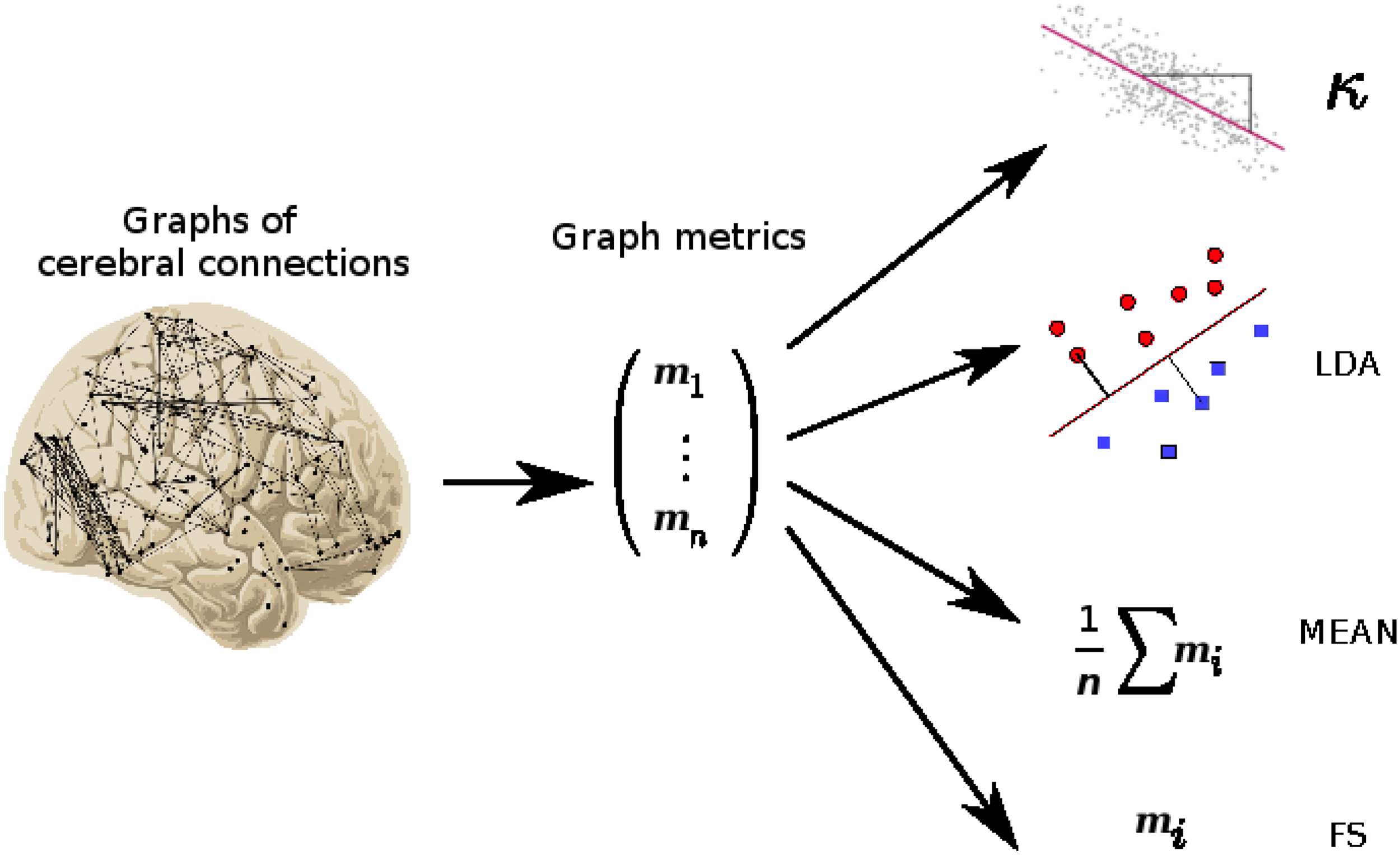
particular property of the data. Cifra 1 gives an illustration of the different methods.
κ Index Definition
In our previous study (Achard et al., 2012), κ was devised to compare graph metrics obtained
on each node of a subject or of a group with a reference group (ver figura 2).
In classical
comparisons between a group of patients and a group of healthy volunteers, the reference
is the group of healthy volunteers. En el presente estudio, for a given graph metric and two
grupos, we first compute the average of this metric for each node over the group of healthy
volunteers, denoted as the reference. Each subject is then summarized as a vector of values
of dimension of the number of nodes. Entonces, for each patient, κ corresponds to the slope of
the regression of a nodal graph metric between the given patient minus the reference and the
yo
D
oh
w
norte
oh
a
d
mi
d
F
r
oh
metro
h
t
t
pag
:
/
/
d
i
r
mi
C
t
.
metro
i
t
.
/
/
t
mi
d
tu
norte
mi
norte
a
r
t
i
C
mi
–
pag
d
yo
F
/
/
/
/
/
5
1
2
5
2
1
9
1
1
5
7
4
norte
mi
norte
_
a
_
0
0
1
7
6
pag
d
.
t
F
b
y
gramo
tu
mi
s
t
t
oh
norte
0
7
S
mi
pag
mi
metro
b
mi
r
2
0
2
3
Cifra 1. General framework from graphs of cerebral connectomes to the different scalar features.
Brain connectivity graphs are extracted from fMRI data. Graph metrics are computed at the nodal
level for each subject. The matrices of graph metrics can then be analyzed using different methods:
the hub disruption index based on regression analyses (k); linear discriminant analysis (LDA); aver-
age of metrics (MEAN); and feature selection (FS). Each of these methods allows us to summarize the
graph metric in one scalar for each subject in order to better differentiate the studied populations.
Neurociencia en red
257
Mapping the brain feature space into lower dimensional manifolds
yo
D
oh
w
norte
oh
a
d
mi
d
F
r
oh
metro
h
t
t
pag
:
/
/
d
i
r
mi
C
t
.
metro
i
t
.
/
t
/
mi
d
tu
norte
mi
norte
a
r
t
i
C
mi
–
pag
d
yo
F
/
/
/
/
/
5
1
2
5
2
1
9
1
1
5
7
4
norte
mi
norte
_
a
_
0
0
1
7
6
pag
d
t
.
F
b
y
gramo
tu
mi
s
t
t
oh
norte
0
7
S
mi
pag
mi
metro
b
mi
r
2
0
2
3
Cifra 2. Extraction of hub disruption index κ. (A) Brain connectomes inferred for each subjects.
(B) For each brain connectome, extraction of graph metrics for each region of the brain. (C) Matrix
representation of the graph metrics, where a row corresponds to a subject and a column corre-
sponds to a brain region. (D) Computation of the hub disruption index by regressing the average of
brain metrics of the difference of patients and average of healthy volunteers against the average of
healthy volunteers. The hub disruption index corresponds to the slope coefficient. We give several
illustrations following the sign of this coefficient.
Neurociencia en red
258
Mapping the brain feature space into lower dimensional manifolds
referencia. Let N denote the number of nodes in the graph, np the number of patients, and nc
the number of controls. Dejar (m1, . . . , mnp ) ∈ RN×np denote a matrix of graph metric extracted
given the graphs of patients, for j, 1 ≤ i ≤ np, mj ∈ RN. For each j, mj is equal to one
graph metric such as D, Eglob, or Clust. Let us also define a similar matrix for the controls,
(h1, . . . , hnc ) ∈ RN×nc. Let us define the average metric for controls, for each i, 1 ≤ i ≤ N,
¯hi =
1
nc
nc
∑
j=1
hij.
κ is defined by the following regression:
mi − hi = κ ¯hi + ǫ
i,
(4)
(5)
where ǫ
i is the classical error term in linear regression. In order to give a simple interpretation
of κ, we assume that the global graph metric computed as an average over the nodes is the
same in both groups. Un valor de 0 for κ is showing that the graph metric obtained at the node
level is the same for the patient and the reference. A positive value of κ is indicating that the
hubs and non-hubs of the patient in comparison to the reference are located on the same
nodos. Sin embargo, the values of the graph metrics are increased for the hubs and decreased for
the non-hubs. Finalmente, when the value of κ is negative, the hubs of the reference are no longer
hubs of the patient, and the non-hubs of the reference are hubs for the patient. In Achard
et al. (2012), we showed that the κ index is able to discriminate both groups (coma patients
and healthy volunteers) while the global metric is unable to identify any significant difference.
Instead of averaging the graph metrics, the κ index is capturing a joint variation of the metrics
computed for each node.
Mean Over the Nodes (MEAN)
For each graph metric, the mean over the nodes of the graph captures a global property of
la red. These global metrics have been previously used to discriminate two populations
of networks, for example for Alzheimer’s disease (Supekar et al., 2008) and for schizophrenia
(Lynall et al., 2010). Such a coefficient can discriminate two networks well when their topolo-
gies are really different. Sin embargo, such metrics do not take into account the specificity of the
nodos. En efecto, when permuting the nodes of the graph, the global metric is not changed, pero
the hubs of the graph are not associated with the same nodes anymore. Por lo tanto, a graph
reorganization cannot be detected using such global metrics.
Linear Discriminant Analysis (LDA)
LDA (Pescador, 1936) is a classification method that aims to aiming at identify the linear projec-
tion optimally separating two groups. It can be considered a gold standard for linear group
discriminación. It is not specific to the analysis of networks.
LDA has been previously used for network discrimination in Robinson et al. (2010). Este
algorithm amounts to computing a scalar for each graph. Sin embargo, there is no simple clinical
interpretation of the discriminating parameter.
Feature Selection (FS)
As for LDA, FS determines the features yielding the best separation of the two groups. Varios
features may be used simultaneously. In order to establish a fair comparison with the other
métodos, we choose to extract the single feature yielding the best separation. Several methods
Neurociencia en red
259
yo
D
oh
w
norte
oh
a
d
mi
d
F
r
oh
metro
h
t
t
pag
:
/
/
d
i
r
mi
C
t
.
metro
i
t
.
/
/
t
mi
d
tu
norte
mi
norte
a
r
t
i
C
mi
–
pag
d
yo
F
/
/
/
/
/
5
1
2
5
2
1
9
1
1
5
7
4
norte
mi
norte
_
a
_
0
0
1
7
6
pag
d
t
.
F
b
y
gramo
tu
mi
s
t
t
oh
norte
0
7
S
mi
pag
mi
metro
b
mi
r
2
0
2
3
Mapping the brain feature space into lower dimensional manifolds
exist for FS. We choose univariate FS implemented in Pedregosa et al. (2011). An advantage
of FS is that it is capturing discriminative features at the node level. As the selected features
are extracted directly from the data, it is usally possible to derive a clinical interpretation.
Sin embargo, joint variations are not modeled, and on the comatose study FS is not able to yield
results of the same quality as those obtained using κ.
Modeling Populations of Networks with Manifold Learning
ISOMAP (Tenenbaum et al., 2000) is used as a manifold learning approach to describe pop-
ulation networks. We propose an original approach based on ISOMAP, where we constrain
one variable of the reduced space (the latent space) to correspond to a covariate.
ISOMAP devises a reduced-dimension version of the orig-
Manifold learning using ISOMAP.
inal set of points. Interpoint distances in the reduced space reproduce as much as possible
interpoint distances in the original space. Euclidean and geodesic distances are respectively
usado. Principal component analysis may be seen as a particular case of ISOMAP, where Eu-
clidean distances are used in the original space, instead of geodesic distances. The reader is
referred to Tenenbaum et al. (2000) for details about the algorithm.
En nuestro caso, the original data correspond to a vector of graph metrics for each subject,
the dimension of the vector being the number of nodes times the number of metrics. Para cada
análisis, only one metric is considered here. Sin embargo, this method could be applied by jointly
using several metrics. Covariates may be regressed on the reduced space. In the present work,
this was achieved using a classic radial basis function interpolation.
The choice of the ISOMAP is twofold: Primero, the estimated reduced space is a smooth man-
ifold, and preserves the global structure of the dataset. Notablemente, the reduced space exhibits a
continuum function of subjects. Segundo, the cost function of the ISOMAP allows the integra-
tion of additional constrained scores. ISOMAP was performed by computing a nearest neigh-
bor graph connecting the four nearest neighbors according to the Euclidean distance. Este
distance correctly reflects the local topology of the graph metrics space. The choice of four
neighbors is driven by the relatively small number of subjects in the study.
The classification score of the ISOMAP was computed using a nonlinear support vector ma-
chine (SVM) approach with radial basis function kernel in the reduced space (Hearst, Dumais,
Osuna, Platón, & Scholkopf, 1998).
Covariate constrained manifold learning. One drawback of manifold learning algorithms is the
difficulty of interpreting the reduced coordinates because they are usually meaningless. El
original method proposed in this work consists of constraining one coordinate of the reduced
space to correspond to a specific covariate. The other coordinates are left unconstrained, como en
classical ISOMAP. Such a procedure requires special care regarding the optimization aspect.
We apply a strategy proposed in Brucher, Enrique, Heitz, and Armspach (2008), where points
are introduced one by one.
Además, a scale factor α is considered for the axis corresponding to the covariate. Este
parameter, obtained by optimization, balances the scales of the different axes.
Neurociencia en red
260
yo
D
oh
w
norte
oh
a
d
mi
d
F
r
oh
metro
h
t
t
pag
:
/
/
d
i
r
mi
C
t
.
metro
i
t
.
t
/
/
mi
d
tu
norte
mi
norte
a
r
t
i
C
mi
–
pag
d
yo
F
/
/
/
/
/
5
1
2
5
2
1
9
1
1
5
7
4
norte
mi
norte
_
a
_
0
0
1
7
6
pag
d
.
t
F
b
y
gramo
tu
mi
s
t
t
oh
norte
0
7
S
mi
pag
mi
metro
b
mi
r
2
0
2
3
Mapping the brain feature space into lower dimensional manifolds
The reduced point ˜xi is defined by ˜xi = [αci; xi]t, where ci is the chosen covariate and xi
are the other coordinates. The cost function E is defined as
E = ∑
i,i
